This is an overview of methods used to design scaled laser experiments to study astrophysical problems – an area of research at AWE which involves the state-of-the-art Orion laser. The article covers analytical methods and large multi-dimensional radiation-hydrodynamic simulations.
1. Introduction
Material in the high-energy-density (HED) state is common in many areas of astrophysics including solar and planetary physics [1], where direct measurements are not possible, and involves temperatures of millions of degrees centigrade, pressures of millions of bars and densities up to hundreds of g/cc. Materials at such conditions enter the plasma regime where atoms collide with sufficient energy to strip electrons away from the nucleus to form a gas of charged ions and free electrons. And when these very energetic electrons decay back down they radiate X-rays.
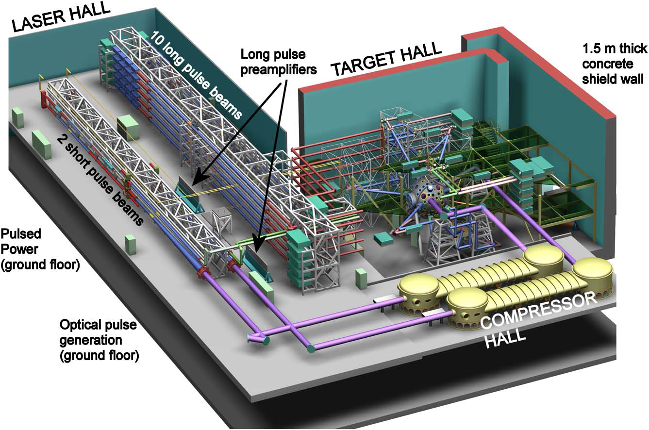
The HED regime is complex and is difficult to access but over the last 50 years various experimental tools have become available to make laboratory experiments possible. High-power lasers like the 5 kJ 12-beam Orion facility at AWE (Figure 1) [2] are one such tool and they achieve high-energy densities by using the temporal and spatial compression of energy to generate fluxes  W/cm
W/cm typically.
Photons do not repel each other and so they can be focussed into small volumes, hence providing the spatial compression. The temporal compression is provided by using stored electrical energy to rapidly energise a lasing medium through which a very-short-duration light pulse (e.g.  sec) is passed to amplify it to very high intensities. Laser energy is of no direct use for HED experiments and so it must be converted to other forms. It can be converted to kinetic energy by irradiating a foil, which ablates material and generates a reactive force that drives a high-pressure shock wave into the bulk material. It can be converted to X-rays by irradiating the inside of a high-atomic-number (e.g. gold) cavity, known as a hohlraum (Figure 2) [3]. The laser light is efficiently absorbed at the wall where material is heated sufficiently to radiate a large proportion of the absorbed energy as X-rays. This heats other wall areas and these reradiate similarly, and so the X-ray field is partially trapped and smoothed, and can be used to drive an experimental package mounted from the wall. The final method is to use ultra-high laser intensities (
 W/cm) to accelerate energetic particles [4] that heat a package directly or via the induced electrical return currents, although this is not discussed further in this article.

Spatial and temporal compression means that laser target sizes are small ( —
— mm typically) and experimental durations are short (
 –
– sec typically). This makes target manufacture and diagnosis challenging.
2. Radiation-hydrodynamic simulations
Complex simulation codes have been developed to model laser targets and the coupling between different physical processes. The workhorse codes are continuum fluid hydrocodes onto which numerous modular physics packages are added to model laser absorption, X-ray transport, etc. The fluid approximation assumes that collisions between atoms/electrons dominate to force local thermodynamic equilibrium and so plasma properties can be described by macroscopic quantities such as temperature and pressure, which is a reasonable approximation for many HED plasmas. Many of the physics packages involve solving coupled non-linear partial differential equations, and for the fluid dynamics these are the three Euler hydrodynamic equations [5] that represent conservation of mass, momentum and energy:
![\begin{align*} \frac{\partial \rho}{\partial t} + \boldsymbol{\nabla}.(\rho \vect{v}) &= 0 \\ \rho \left[\frac{\partial \vect{v}}{\partial t} + (\vect{v}.\boldsymbol{\nabla})\vect{v})\right] &= -\boldsymbol{\nabla} P \\ \frac{\partial(\rho E)}{\partial t} + \vect{v}.\boldsymbol{\nabla}(\rho E) &= -(\rho E + P)\boldsymbol{\nabla}.\vect{v}. \end{align*}](https://ima.org.uk/wp/wp-content/ql-cache/quicklatex.com-2a090654fa16fd32134b3cb752de80d1_l3.svg "Rendered by QuickLaTeX.com")
These three equations in four unknowns, density  , pressure
  , velocity
  and specific internal energy
  , are supplemented by material equations-of-state (EoS) that give from and to allow the system to be solved. Fluid viscosity is not represented in the above equations because it is usually small for HED plasmas.
Laser targets are designed using 1D, 2D and 3D radiation-hydrodynamic simulations like the example shown in Figure 3. Modelling is limited by computer power which has been increasing rapidly, with AWE resources increasing from 0.1 teraflop/s in 1998 to 4000 teraflop/s in 2016. This now allows 2D and increasingly 3D simulations to be routine, which is important because most laser targets have significant 2D and 3D features. These large increases in computing power have been achieved through massively parallel processing with large simulations run over thousands of processors. This requires codes to have good load balancing between processors with minimised processor-to-processor communications because this is relatively slow.

Traditionally fluid dynamics is solved with either Lagrangian hydrodynamics where the computational mesh is anchored to the material (Figure 3), or Eulerian hydrodynamics where the mesh is fixed in space with material advected from cell to cell. Subzone interface reconstruction is very important for Eulerian hydrodynamics to ensure materials are advected accurately with little numerical diffusion, although some dissipation is inevitable. Lagrangian hydrodynamics maintains material interfaces precisely but mesh distortion can become a problem leading to poor accuracy (e.g. mesh imprint) and possibly simulation failure. Lagrangian methods are more efficient with fine zoning focused in important regions to resolve laser and X-ray interactions and so it is frequently beneficial to model a laser target with Lagrangian hydrodynamics initially and then map to Eulerian at later times when the mesh starts to tangle.
The distinction between Lagrangian and Eulerian is now blurring with the introduction of arbitrary Lagrangian–Eulerian (ALE) codes, where Lagrangian and Eulerian regions coexist with Eulerian hydrodynamics applied to areas where shear flows are high, while retaining the efficiency of Lagrangian hydrodynamics elsewhere. An alternative approach to ALE is adaptive mesh refinement (AMR) where Eulerian hydrodynamics is used globally with patches of increasing mesh refinement applied based on local gradients to better resolve physical processes. Even the distinction between AMR and ALE codes could disappear with AMR potentially included in ALE codes. Hydrodynamics is modelled explicitly with a global time step, governed by the fastest cell-to-cell communication based on the local sound speed to ensure stability (i.e. Courant–Friedrichs–Lewy condition [6]). Finite-difference methods (with artificial viscosity to smear shock discontinuities) have been used extensively [6] but these are now evolving to finite-element schemes and potentially high-order Godunov methods [7].
Any element in a hot body emits X-ray radiation based on its temperature  , density and its radiative opacity
  , where opacity is the opaqueness of the material to photons and sets transmission through an element of thickness
  as
as  . These photons then propagate and are absorbed or amplified by the surrounding material. This propagation obeys the radiation transport equation, which is a form of the Boltzmann transport equation [8],
![\begin{multline*} \frac{1}{c} \frac{\partial I(\vect{r},t,\upsilon,\boldsymbol{\Omega)}}{\partial t} + \boldsymbol{\Omega}.\boldsymbol{\nabla} I(\vect{r},t,\upsilon,\boldsymbol{\Omega}) =\\ \rho(\vect{r},t)\kappa (\vect{r},t,\upsilon)[B(\vect{r},t,\upsilon)-I(\vect{r},t,\upsilon,\boldsymbol{\Omega})] \end{multline*}](https://ima.org.uk/wp/wp-content/ql-cache/quicklatex.com-06dfe70ccce04f7a5577212e92b580f2_l3.svg "Rendered by QuickLaTeX.com")
where  is the specific intensity at position
  and photon frequency
  , along vector direction
  within solid angle
  ,
,  is time,
  is the speed of light, and
  is the local emission source, which is the Planck function [8] if local thermodynamic equilibrium is assumed. This can be solved using a range of methods.
For optically thick systems such as a hohlraum wall, where there is continual strong absorption and isotropic re-emission of X-rays, the solution can be approximated by diffusion [8], with the flux of radiation energy proportional to the gradient in temperature,  (like thermal conduction), where
  is the diffusion coefficient, which is
  , with
  the Stefan–Boltzmann constant and
  is a weighted integral of the frequency-dependent opacity known as the Rosseland average [8].
Numerical diffusion solutions are fast and spatially smooth although the diffusion approximation is inappropriate for many situations of interest such as optically thin plasmas, where photons can free-stream or where an opaque wall (e.g. hohlraum) constrains the X-ray flow (e.g. radiation diffusion flows around an opaque obstruction with no representation of shadowing effects). In such cases a full transport solution is needed with the most common being statistical Monte Carlo methods where emission is approximated by particles, each representing a huge number of photons, and these are generated randomly based on the local material properties [9].
The most common alternative to Monte Carlo is deterministic SN [8], also known as discrete ordinate, where fixed quadrature sets (e.g. Gauss–Legendre) define discrete directions covering a unit sphere (from each mesh cell) along which the radiation transport equation is solved. Monte Carlo is typically less expensive than SN for modelling laser targets but suffers from statistical noise, which can make it unsuitable for modelling hydrodynamic instabilities, whereas SN can suffer from ray effects if the quadrature set is not of high enough order. Monte Carlo and SN require efficient solutions for ray interceptions with the fluid mesh, and diffusion requires fast matrix inversions.
An explicit radiation scheme would require a very small simulation time step (e.g.  sec) in order to resolve the mutual communication between cells based on the speed of light. This is impractical for multi-dimensional simulations so an implicit scheme is typically used which is universally stable, although this does not guarantee accuracy. For Monte Carlo the implicit feedback during a time step is achieved by treating absorption as pseudo-scattering [9], where the local conditions make this
reasonable such as hot opaque material. This assumes the absorbed energy is immediately reradiated isotropically with characteristics changed to those of the local material.
Radiation-hydrodynamic modelling is fundamentally dependent on material properties data over a wide range of density and temperature space. The main inputs are equation-of-state (i.e. internal energy and pressure for a given density and temperature) and opacity. These are typically interpolated from large grids generated offline by detailed atomic physics and thermodynamic codes.
3. Analytical theory
Much of the initial design work for laser targets can be done with analytical models, especially if the basic target evolution is 1D. Hydrodynamics is well understood and analytical solutions of the Euler equations exist for a variety of phenomena of interest such as shock compression and adiabatic expansions [10], and these can be coupled together (e.g. release adiabatic following a shock). Tabulated EoS are inconvenient for analytical work but fortunately it is often reasonable to approximate a plasma as a polytropic fluid [5], where pressure  with
with  the adiabatic index derived by best fitting to an EoS over the regime of interest [10]. A perfect gas of
  is reasonable for hot low-atomic-number materials although smaller values are more appropriate (e.g. 1.3) for cooler conditions where molecular dissociation and ionisation energies are more significant, robbing energy from pressure generation.
For some analytical models then more complex EoS forms can be used or a model may require additional data such as opacities, and power-law fits (e.g.  ) to the tabulated data are often suitable in these cases. 1D radiation-hydrodynamic simulations are often run purely to obtain compendia of formulae for how one physical quantity varies as the drive is changed (e.g. shock pressure generated for a given laser irradiance). These can then be used to assess quickly possible ablator designs, etc.
The design of hohlraums is an area where analytical models are used extensively for initial scoping studies. X-ray emission from the laser spots drives a heatwave into other wall areas and the speed of this wave governs how well the cavity contains the energy. The heatwave in a gold hohlraum is diffusive (as discussed in Section 2) with a coefficient that is very sensitive to temperature with a further large sensitivity introduced from a strong temperature dependence in the opacity . This makes the problem highly non-linear resulting in a very steep gradient at the heatwave front and makes analytical solutions challenging, however, various exact and approximate solutions can be derived for many cases [11]. The laser-spot X-ray sources can be combined with diffusive wall losses and other losses (e.g. hohlraum holes) in a simple power-balance equation to derive the time-dependent average drive temperature.
For a perfect hohlraum then the X-ray flux would be the same at all points giving perfect drive uniformity, however, this is never achieved because of the finite laser spots, which are hotter than their surroundings, and the laser entrance holes. To ensure good drive uniformity then the laser beams must be carefully positioned to minimise drive variations over the experimental package and the quickest way to assess this is with view-factors analysis [12], which gives radiative coupling coefficients between different wall areas. This is a standard technique for applied heat-transfer problems (e.g. grill design in a domestic cooker) and compendia of object-to-surface coupling formulae are published or can be calculated with area integrals [12].
4. Instabilities
Instability growth at material interfaces is a major concern for many laser targets since it occurs as a direct result of the strong accelerations that are often essential to drive material into the HED state. This mixing of materials can degrade measurement accuracies and in the worst cases compromise an experiment. The main types are the Rayleigh–Taylor (RT) instability, which occurs when a lower density material accelerates a higher density material (i.e. the low-density fluid is accelerated more strongly and so penetrates the denser fluid); the Richtmyer–Meshkov instability, where a shock wave passes through an interface between materials of different densities (i.e. impulsive form of RT); and the Kelvin–Helmholtz instability, where there is shear flow of one fluid over another (e.g. wave generation at sea by wind) [1].
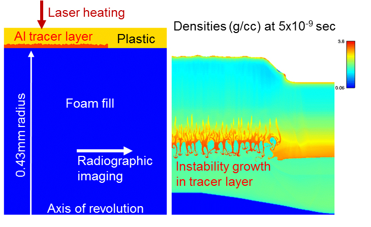
The RT instability is of greatest concern since wavelength modes grow exponentially (with time) and independently during the initial linear phase. As amplitudes exceed  times the mode wavelength their growth rate reduces as mode coupling and fluid drag divert energy to other wavelengths. With acceleration over sufficient distance then this can develop into full turbulence with a self-similar Kolmogorov cascade of turbulent kinetic energy from the longer driven modes to shorter wavelengths and then to viscous heat dissipation at small scales [13]. The RT instability also occurs at the ablation front of any accelerated foil [3] because this is where hot low-density plasma accelerates the dense bulk foil, although ablation reduces growth rates since RT modulation spikes are exposed to heating over a greater surface area, and this polishing is greatest for shorter wavelengths. Instabilities can be controlled by minimising density discontinuities in the target and by reducing surface roughness at material interfaces in target fabrication. Modelling of typical instability growth is shown in Figure 4.
The desire to achieve the highest HED conditions often means accepting some instability growth and so considerable effort is devoted to large 2D and 3D radiation-hydrodynamic simulations of material mixing to ensure growth is acceptable. This is supported by experiments conducted specifically to validate modelling of instability growth and mixing, and related campaigns are also done because instability growth is important in many astrophysical objects (e.g. supernova explosions [1]). Explicit 3D modelling of turbulence covering all scale lengths to viscous dissipation is usually impractical, even with current computing resources, and so simplified approaches are used such as large-eddy simulations [13], and such approximations require validation.
5. Scaling and an example astrophysical experiment
Laser experiments to study an astrophysical object typically try to preserve dimensionless numbers that are characteristic of the important physics (e.g.\ Mach number). Euler scaling [14] is used for the hydrodynamics where sizes, densities, pressures and timescales are scaled like in a wind-tunnel trial. The Euler equations in Section 2 with the additional assumption of a polytropic EoS, , remain invariant under the following transformations where  ,
,  and are scaling constants:

By constructing a laser target that is a miniature replica of the astrophysical object with scaled dimensions and densities then this fixes and . Pressure is then set by the available laser driver and this then defines the timescale of the experiment. The final requirement is to use materials in the laser experiment whose adiabatic indices at the scaled conditions are close to the astrophysical materials at their conditions. The scaled system will then evolve similarly.

Pure Euler scaling requires that both fluid viscosity and heat exchange are negligible, however, X-ray transport is often important in astrophysical objects [1], changing the hydrodynamics, and laser experiments to study this and other effects like magnetic fields need to scale these aspects also. This is possible in many cases [15] although relaxing some scaling requirements can often give a simpler experiment. Material data and target fabrication uncertainties usually introduce the largest errors in scaled experiments and these need to be minimised, possibly by conducting supporting EoS tests. Larger laser facilities are usually advantageous because they can drive larger targets, which are easier to manufacture and diagnose, to conditions that are closer to the astrophysical object.
A recent experiment was conducted on the Orion laser to mimic supersonic plasma falling into the polar region of a white-dwarf star along strong magnetic field lines and generating a strong reverse shock from the surface impact [16, 17]. This astrophysical case was scaled to the experiment shown in Figure 5 with the laser used to accelerate a plastic foil which unloads as a hot plasma down a plastic tube used to represent the constraining effects of the magnetic fields. The flow stagnates against a metal anvil and produces a return shock akin to the accretion shock in the astrophysical system. Radiographic imaging data are matched by simulation (Figure 5), which helps validate the accuracy of the radiation-hydrodynamic code for application to the astrophysical object.
6. About AWE
The Atomic Weapons Establishment plays a crucial role in our nation’s defence by providing and maintaining warheads for Trident, the UK’s nuclear deterrent. AWE has proudly been at the forefront of the UK’s nuclear deterrence programme for over 60 years and delivers innovative solutions to safeguarding national nuclear security. For further information visit AWE.co.uk
Peter Graham
Atomic Weapons Establishment (AWE), Aldermaston
References
- Drake, R.P. (2006) High-Energy Density Physics, Springer, New York.
- Hopps, N. et al. (2013) Overview of laser systems for the Orion facility at the AWE, Appl. Opt., vol. 52, no. 15, pp. 3597–3607.
- Lindl, J. (1995) Development of the indirect-drive approach to inertial confinement fusion and the target physics basis for ignition and gain, Phys. Plasmas, vol. 2, no. 11, pp. 3933–4024.
- Gibbon, P. (2005) Short Pulse Laser Interactions with Matter, Imperial College Press, London.
- Landau, L.D. and Lifshitz, E.M. (1987) Fluid Mechanics, 2nd edition, Pergamon Press, Oxford.
- Woolfson, M.M. and Pert, G.J. (1999) An Introduction to Computer Simulation, Oxford University Press, Oxford.
- Barlow, A.J. and Roe, P.L. (2011) A cell-centred Lagrangian Godunov scheme for shock hydrodynamics, Comput. Fluids, vol. 46, pp. 133–36.
- Pomraning, G.C. (2005) Radiation Hydrodynamics, Dover, New York.
- Fleck, J.A. and Cummings, J.D. (1971) An Implicit Monte Carlo Scheme for calculating time and frequency dependent nonlinear radiation transport, J. Comput. Phys., vol. 8, pp. 313–42.
- Zel’dovich, Ya.B. and Raizer, Yu.P. (2002) Physics of Shock Waves and High-Temperature Hydrodynamic Phenomena, Dover, New York.
- Hammer, J.H. and Rosen, M.D. (2003) A consistent approach to solving the radiation diffusion equation, Phys. Plasmas, vol. 10, no. 5, pp. 1829–45.
- Incropera, F.P. and De Witt, D.P. (1990) Fundamentals of Heat and Mass Transfer, 3rd edition, Wiley, Hoboken.
- Pope, S.B. (2000) Turbulent Flows, Cambridge University Press, Cambridge.
- Ryutov, D. et al. (1999) Similarity criteria for the laboratory simulation of supernova hydrodynamics, Astrophys. J., vol. 518, pp. 821–32.
- Bouquet, S. et al. (2010) From lasers to the universe: scaling laws in laboratory astrophysics, High Energy Density Phys., vol. 6, pp. 368–80.
- Falize, E. et al. (2012) High-energy density laboratory astrophysics studies of accretion shocks in magnetic cataclysmic variables, High Energy Density Phys., vol. 8, pp. 1–4.
- Cross, J.E. et al. (2016) Laboratory analogue of a supersonic accretion column in a binary star system, Nat. Commun., vol. 7, p. 11899.
Reproduced from Mathematics Today, February 2017
Download the article, Laser Experiments for Astrophysics (pdf)


