When Jordan Spieth failed to make the green on the 12th at Augusta in 2016 and saw his ball plunge into the lake, his dismay was perhaps tempered by the beautifully symmetric ripples or waves emanating from the point where the ball entered the water. An example of such a splash can be seen in Figure 1.

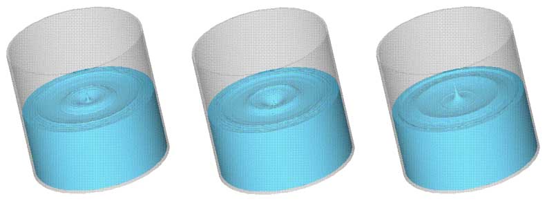
This is a classical free surface fluid mechanics problem involving the Navier–Stokes equations together with the conservation of mass. These may be solved by a variety of methods. We choose a finite difference method employing marker and cell (MAC method) on a staggered grid, which we have been developing over many years. A review of the MAC method may be found in [1]. Figure 2 displays the numerical solution of a splashing drop at three different times using the MAC method (albeit, in a confined region with wave reflection). Note that in Figure 1, a series of concentric crests and troughs are observed whose amplitudes are not constant, nor are the distances between the crests.
It is, however, well known but nonetheless somewhat surprising that substantial progress may be made analytically using asymptotic arguments. In the remainder of this note we shall show how using Hankel transforms, the method of stationary phase and asymptotic analysis, can lead to a simple analytic expression which encapsulates the main features of the flow and indeed compares tolerably with the computation of Figure 2.
An asymptotic expression
In cylindrical polar coordinates with  -axis vertically upwards, the linearised water wave equations are
 where
where  denotes the elevation (above
  ) of the water and
  is the velocity potential (i.e.
  ). See, e.g. Coulson [2].
Note that from Jordan Spieth’s point of view, time is initiated, not when his ball hits the water, but at the time when the resultant splash occurs.
Define the Hankel transforms

Taking Hankel transforms of (1) yields
![\[ \frac{\partial^2 \tilde \phi}{\partial z^2} - k^2 \tilde \phi = 0 \]](https://ima.org.uk/wp/wp-content/ql-cache/quicklatex.com-ffe2bbe048b8ef064fe50d956b5fd9a5_l3.svg "Rendered by QuickLaTeX.com")
or, using (4),
(6) 
Equations (2) and (3) provide
(7) 
whence
![\[ \frac{\partial^2 A}{\partial t^2} + g|k| A = 0 \]](https://ima.org.uk/wp/wp-content/ql-cache/quicklatex.com-a9b9534270d0f9b55f9df49483c92b20_l3.svg "Rendered by QuickLaTeX.com")
and so
![\[ A(k, t) = a(k) \mathrm{e}^{\mathrm{i} wt} + b(k) \mathrm{e}^{-\mathrm{i}wt}, \ w^2 = g|k|. \]](https://ima.org.uk/wp/wp-content/ql-cache/quicklatex.com-3c2668f32479742104743f67d7226e7c_l3.svg "Rendered by QuickLaTeX.com")
Substituting back into (6) then gives
![\[ \tilde\phi (k, z, t) = \left[ a(k) \mathrm{e}^{\mathrm{i}wt} + b(k) \mathrm{e}^{-\mathrm{i}wt} \right]\mathrm{e}^{|k|z}. \]](https://ima.org.uk/wp/wp-content/ql-cache/quicklatex.com-ce8c59eb98116abbda0dee243029f5a2_l3.svg "Rendered by QuickLaTeX.com")
However,
![\[ \tilde\phi = 0 \quad \mbox{when} \quad t = 0 \]](https://ima.org.uk/wp/wp-content/ql-cache/quicklatex.com-cdbb2ac6911755c4e7b1d5149e51e702_l3.svg "Rendered by QuickLaTeX.com")
and so
![\[ \tilde \phi (k, z, t) = a(k) (\mathrm{e}^{\mathrm{i}wt} - \mathrm{e}^{-\mathrm{i}wt}) \mathrm{e}^{|k|z}. \]](https://ima.org.uk/wp/wp-content/ql-cache/quicklatex.com-11ab03dd7afd139a50c203fbf50d0762_l3.svg "Rendered by QuickLaTeX.com")
Moreover, substitution into the Hankel transform of (2) results in
(8) 
However,
![\[ \tilde\zeta (k, t) = \tilde \zeta_0 (k) \]](https://ima.org.uk/wp/wp-content/ql-cache/quicklatex.com-44585226280bcfda9fa176845b441a3f_l3.svg "Rendered by QuickLaTeX.com")
when  and so
![\[ a(k) = -\frac{\mathrm{i}g \tilde\zeta_0 (k)}{2w}. \]](https://ima.org.uk/wp/wp-content/ql-cache/quicklatex.com-f80585d8e80ab0d04fc0037fc8a2802d_l3.svg "Rendered by QuickLaTeX.com")
Thus, from (8), we have
![\[ \tilde\zeta (k, t) = \frac{1}{2} (\mathrm{e}^{\mathrm{i}wt} + \mathrm{e}^{-\mathrm{i}wt}) \tilde\zeta_0 (k). \]](https://ima.org.uk/wp/wp-content/ql-cache/quicklatex.com-6d040fc18168169675b7299842e0aa04_l3.svg "Rendered by QuickLaTeX.com")
Taking the inverse Hankel transform results in
![\[ \zeta (r, t) = \int^\infty_0 kJ_0 (kr) \cos wt\, \tilde \zeta_0 (k) \mathrm{d} k \]](https://ima.org.uk/wp/wp-content/ql-cache/quicklatex.com-f9ca6652e73df015e6100186458d25e7_l3.svg "Rendered by QuickLaTeX.com")
where
![\[ \tilde\zeta_0 (k) = \int^\infty_0 r\, J_0 (kr) \zeta_0 (r) \mathrm{d} r. \]](https://ima.org.uk/wp/wp-content/ql-cache/quicklatex.com-f5be4a3ef76fd8a502d0f6768fc7998c_l3.svg "Rendered by QuickLaTeX.com")
Let us define the initial disturbance to be
(9) 
at time .
Then
![\[ \tilde\zeta_0 (k) = a\int^\rho_0 r\, J_0 (kr) \mathrm{d} r = \frac{a\rho}{k}\, J_1 (k\rho). \]](https://ima.org.uk/wp/wp-content/ql-cache/quicklatex.com-f6d890a224c1af7d3cb3b962ba79344b_l3.svg "Rendered by QuickLaTeX.com")
Therefore
(10) 
The integral form of the Bessel function is
![\[ J_0 (kr) = \frac{2}{\pi} \int^{\pi/2}_0 \cos (kr \cos \theta) \mathrm{d}\theta. \]](https://ima.org.uk/wp/wp-content/ql-cache/quicklatex.com-3221f39e9d7191d88ebfc3ae9fa7355e_l3.svg "Rendered by QuickLaTeX.com")
We may therefore express (10) as follows:
(11) 
where  denotes the real part of the double integral.
Interchange the order of integration and define
(12) ![\begin{equation*} k(\theta) = \int^\infty_0 J_1 (k\rho) \left[\mathrm{e}^{\mathrm{i}(wt + kr \cos \theta)} + \mathrm{e}^{\mathrm{i}(-wt + kr \cos \theta)}\right] \mathrm{d} k. \end{equation*}](https://ima.org.uk/wp/wp-content/ql-cache/quicklatex.com-a028c447d6432cc088c8a1a58b022484_l3.svg "Rendered by QuickLaTeX.com")
With the change of variables  and
and  , then (12) becomes
(13) ![\begin{equation*} k(\theta) =\frac{2}{\rho} \int^\infty_0 J_1 (p^2) \left[\mathrm{e}^{\mathrm{i}(p^2 \cos \theta + 2p \tau)r/\rho} + \mathrm{e}^{\mathrm{i}(p^2 \cos \theta - 2p\tau)r/\rho}\right] p \mathrm{d} p. \end{equation*}](https://ima.org.uk/wp/wp-content/ql-cache/quicklatex.com-411bda00a601c1531f5943bcb5719fc8_l3.svg "Rendered by QuickLaTeX.com")
Here we assume  . In this case, the trigonometric functions will vary extremely rapidly from
  to
to  with the positive and negative components cancelling each other out. This will happen except where the function
  is stationary in the interval of integration. We observe that this will not be the case for
  since the stationary point is outside the range of integration. Thus the leading order term in (13) is the second (and consequently the first may be neglected). Furthermore
![\[ f' (p) = 2p \cos \theta - 2\tau \]](https://ima.org.uk/wp/wp-content/ql-cache/quicklatex.com-a867d95b32026b3375d355e89c22b122_l3.svg "Rendered by QuickLaTeX.com")
implying that the stationary point  is
is
![\[ p_0 = \tau/\cos \theta. \]](https://ima.org.uk/wp/wp-content/ql-cache/quicklatex.com-08d0437aac07950ad6d6538c8dcfaa59_l3.svg "Rendered by QuickLaTeX.com")
Excluding  in the neighbourhood of
  , we may write
![\[ f(p) = [(p - p_0)^2 - p^2_0] \cos \theta. \]](https://ima.org.uk/wp/wp-content/ql-cache/quicklatex.com-963609209d137eb7b56a73bf0794b270_l3.svg "Rendered by QuickLaTeX.com")
Then the integral (13) may be approximated by
![\begin{align*} k(\theta) &\sim \frac{2}{\rho} \int^{p_0 +\epsilon}_{p_0-\epsilon} J_1 (p^2) \\ & \qquad \exp \left[\mathrm{i}\left(\cos \theta \, (p-p_0)^2 \frac{r}{\rho} - \cos \theta \, p^2_0 \frac{r}{\rho} \right)\right] p \mathrm{d} p \\ &= \frac{2}{\rho} \exp \left(-\mathrm{i}\cos \theta \, p^2_0 \frac{r}{\rho}\right) \\ & \qquad \int^{p_0 +\epsilon}_{p_0-\epsilon} J_1 (p^2) \exp \left[\mathrm{i}\cos \theta \, (p-p_0)^2 \frac{r}{\rho}\right] p \mathrm{d} p, \end{align*}](https://ima.org.uk/wp/wp-content/ql-cache/quicklatex.com-23659cbac056960d9164898f2d0fe327_l3.svg "Rendered by QuickLaTeX.com")
with the integral outside the range ![[p_0 - \epsilon, p_0 + \epsilon]](https://ima.org.uk/wp/wp-content/ql-cache/quicklatex.com-96a3a9c7c906147671d1257c120978be_l3.svg "Rendered by QuickLaTeX.com") cancelling to zero.
cancelling to zero.
The factors  and
and  are slowly varying compared with the rapidly fluctuating cosine and sine functions and so may be replaced by and
  , respectively.
Thus
![\begin{multline*} k(\theta) \sim \frac{2}{\rho} \exp \left[-\mathrm{i}\cos \theta\, p^2_0\, \frac{r}{\rho}\right] p_0 J_1 (p^2_0) \\ \int^{p_0 +\epsilon}_{p_0-\epsilon} \exp \left[\mathrm{i}\cos \theta \, (p-p_0)^2 \frac{r}{\rho}\right] \mathrm{d} p. \end{multline*}](https://ima.org.uk/wp/wp-content/ql-cache/quicklatex.com-b20f439d78ddf00dcfbcb5e5121728b2_l3.svg "Rendered by QuickLaTeX.com")
We now make the following further change of variables:
![\[ s = q(p-p_0), \quad q^2 = \frac{r}{\rho} \cos \theta \]](https://ima.org.uk/wp/wp-content/ql-cache/quicklatex.com-093135a5bc9602e8a6a52e4084b25b3f_l3.svg "Rendered by QuickLaTeX.com")
so that
![\[ k(\theta) \sim \frac{2}{\rho} \exp \left[-\mathrm{i}\cos \theta \, p^2_0 \frac{r}{\rho}\right] \frac{p_0}{q}\, J_1 (p^2_0) \int^{q\epsilon}_{-q\epsilon} \mathrm{e}^{\mathrm{i}s^2} \mathrm{d} s. \]](https://ima.org.uk/wp/wp-content/ql-cache/quicklatex.com-c71bc1489ee9e33fa44e5bda41b803fc_l3.svg "Rendered by QuickLaTeX.com")
The limits in the integral can be considered infinite if  , implying
  for a small, but fixed
  assuming
  (that is, excluding in the neighbourhood of ).
Now
(14) ![\begin{equation*} \int^\infty_{-\infty} \mathrm{e}^{\pm \mathrm{i}s^2} \mathrm{d} s = \sqrt{\pi} \mathrm{e}^{\pm \mathrm{i}\pi/4} \quad \mbox{(see [3])} \end{equation*}](https://ima.org.uk/wp/wp-content/ql-cache/quicklatex.com-3b609a3cd0fcffdd5a755bf98b0d7b54_l3.svg "Rendered by QuickLaTeX.com")
so that we may write
![\[ k(\theta) \sim \frac{2\sqrt{\pi}}{\rho} \exp \left[-\mathrm{i}\left(\cos \theta \, p^2_0 \,\frac{r}{\rho} - \frac{\pi}{4}\right)\right] \frac{p_0}{q}\, J_1 (p^2_0). \]](https://ima.org.uk/wp/wp-content/ql-cache/quicklatex.com-9d78af972f5e57b6a926a52774cccc51_l3.svg "Rendered by QuickLaTeX.com")
Furthermore,
![\[ p_0 = \dfrac{t\sqrt{g\rho}}{2r \cos \theta}, \]](https://ima.org.uk/wp/wp-content/ql-cache/quicklatex.com-05cfa3e353928f115cb6716963eaaf91_l3.svg "Rendered by QuickLaTeX.com")
so  when
when  and consequently
  and we can write
(15) ![\begin{equation*} k(\theta) \sim \frac{\sqrt{\pi}}{\rho q}\, p^3_0 \exp \left[-\mathrm{i}\left(\cos \theta \, p^2_0 \frac{r}{\rho} - \frac{\pi}{4}\right)\right]. \end{equation*}](https://ima.org.uk/wp/wp-content/ql-cache/quicklatex.com-49450e0e4d2658c05c7b2544e4be98a9_l3.svg "Rendered by QuickLaTeX.com")
Substituting back into equation (11) results in
(16) ![\begin{equation*} \zeta (r, t) \sim \operatorname{Re} \left\{\frac{a}{\sqrt{\pi}} \int^{\pi/2}_0 \frac{p^3_0}{q} \exp \left[-\mathrm{i}\left(\cos \theta \, p^2_0 \frac{r}{\rho} - \frac{\pi}{4}\right)\right] \mathrm{d}\theta\right\}. \end{equation*}](https://ima.org.uk/wp/wp-content/ql-cache/quicklatex.com-549c7362ef1b23eca2a8d8776f090d92_l3.svg "Rendered by QuickLaTeX.com")
On introducing the volume displaced by the initial pulse  , equation (16) becomes
(17) ![\begin{multline*} \zeta(r, t) \sim \\ \operatorname{Re} \left\{\frac{V_0}{\pi^{3/2} \rho^2} \int^{\pi/2}_0 \frac{p^3_0}{q} \exp \left[-\mathrm{i}\left(\cos\theta \, p^2_0 \frac{r}{\rho} - \frac{\pi}{4}\right)\right] \mathrm{d}\theta\right\}. \end{multline*}](https://ima.org.uk/wp/wp-content/ql-cache/quicklatex.com-c8179c28e443480af6537c5b2e34d039_l3.svg "Rendered by QuickLaTeX.com")
We shall consider  such that
  remains finite (and constant). Introducing a final change of variables
  , (17) becomes
(18) 
We now consider the asymptotic limit as  , i.e.
  , or
, or  .
.
Once again we note that for large  (and ) the integrand oscillates extremely rapidly and so defining
![\[ g(\theta) = u/\cos \theta - \frac{\pi}{4}, \]](https://ima.org.uk/wp/wp-content/ql-cache/quicklatex.com-b8eb454413a844df6904b97d90c01d81_l3.svg "Rendered by QuickLaTeX.com")
we observe that  implies
  . Further
  and so
![\[ g(\theta) \simeq g(\theta_0) + \frac{(\theta - \theta_0)^2}{2!} g'' (\theta_0) = u\left( 1 + \frac{\theta^2}{2}\right) - \frac{\pi}{4}. \]](https://ima.org.uk/wp/wp-content/ql-cache/quicklatex.com-32aa1d42879c82da2557036b17cd0aa8_l3.svg "Rendered by QuickLaTeX.com")
We may therefore replace (18) by
![\[ \zeta (r, t) \sim \operatorname{Re} \left\{\frac{V_0}{r^2} \left(\frac{u}{\pi}\right)^{3/2} \mathrm{e}^{-\mathrm{i}\pi/4}\int^\epsilon_{-\epsilon} \mathrm{e}^{-\mathrm{i}u(1+\theta^2/2)} \mathrm{d}\theta \right\} \]](https://ima.org.uk/wp/wp-content/ql-cache/quicklatex.com-30102bb44a56c992e9c6be0b17daec5e_l3.svg "Rendered by QuickLaTeX.com")
and, since the integral is essentially annihilated (cancels itself out) for  we may write
![\[ \zeta (r, t) \sim \operatorname{Re} \left\{\frac{V_0}{r^2} \left(\frac{u}{\pi}\right)^{3/2} \mathrm{e}^{-\mathrm{i}\pi/4} \int^\infty_{-\infty} \mathrm{e}^{-\mathrm{i}u(1+\theta^2/2)} \mathrm{d}\theta\right\}. \]](https://ima.org.uk/wp/wp-content/ql-cache/quicklatex.com-fc8b13bb344adff30105f43e70d7dc29_l3.svg "Rendered by QuickLaTeX.com")
Note that  for
for ![\theta \in [-\epsilon, \epsilon]](https://ima.org.uk/wp/wp-content/ql-cache/quicklatex.com-cd5f4a1c2db10a87d4945cdee94533ee_l3.svg "Rendered by QuickLaTeX.com") and is slowly varying for
and is slowly varying for  .
.
Thus

since
![\[ \int^\infty_{-\infty} \mathrm{e}^{-\mathrm{i}u\theta^2/2} \mathrm{d}\theta = \sqrt{\frac{2\pi}{u}} \mathrm{e}^{-\mathrm{i}\pi/4}. \]](https://ima.org.uk/wp/wp-content/ql-cache/quicklatex.com-f802e9aa907206993b2860d88bbc9b59_l3.svg "Rendered by QuickLaTeX.com")
Thus, upon taking the real part, we obtain
(19) 
where, recall, .
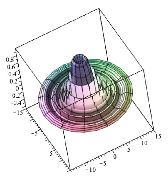

The asymptotic expression (19) for the resulting concentric waves are displayed in Figure 3. It should be stressed that this is only a valid approximation when the fluid velocity is small (i.e.  can be neglected) and when
  and
and  .
.
We note that becomes infinite at (a direct result of letting for a fixed ); however, in Figure 3, a smoothing function has been added for exposition. The amplitudes of the crests decrease according to  or
or  . Furthermore, it is easily seen that the crests follow each other at a distance
  Hence the wavelength is no longer a constant, but increases at constant
  with
with  and decreases at constant
  with
with  .
.
For further reading on the subject and more complicated wave patterns, for example, the wake behind a ship, the reader is referred to [4] and [5].
Sean McKee CMath FIMA
University of Strathclyde
Murilo F. Tomé
University of São Paulo
References
- McKee, S., Tomé, M.F., Ferreira, V.G., Cuminato, J.A., Castelo, A. and Sousa, F.S. (2008) The MAC method, Comput. Fluids, vol. 37, pp. 907–930.
- Coulson, C.A. (1961) Waves, Oliver and Boyd, Edinburgh.
- Spiegel, M.R. (1964) Theory and Problems of Complex Variables, Schaum Publishing Co, NY.
- Whitham, G.B. (1999) Linear and Nonlinear Waves, Wiley, New Jersey.
- Johnson, R.S. (1997) A Modern Introduction to the Mathematical Theory of Water Waves, Cambridge University Press.
Reproduced from Mathematics Today, April 2018
Download the article, Ripples from a Splashing Drop (pdf)
Image credit: Water Drop. Crown, close. © Evan Spiler | Dreamstime.com


