Paint by Number

We start this article with a puzzle: What relates the following? Bisque. Old lace. Burly wood. Chartreuse. Papaya whip.

These seemingly random phrases turn out, disappointingly, to be official names for HTML colours. When did life become so complicated? My sister recalls how she was recently colouring with her 6-year-old godbrother when he proclaimed that his favourite colour is aqua! Does anyone else remember the good old days when we just stuck with the simple red, yellow, green and blue? Well, it turns out that four colours is all one needs.

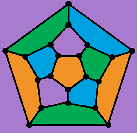
Allow me to clarify. In mathematics, we define a map as a planar¹ representation of a connected, bridgeless graph. Note that this definition encompasses conventional maps too, with the counties/countries/states corresponding to the faces of a graph. We then define a proper face-colouring of a map to be the process of assigning a colour to each face such that any two faces that share an edge are different colours; not forgetting, of course, that the ‘infinite face’ surrounding the outside of the map must be coloured too. You can see such an example in Figure 1 – the dodecahedral graph. It is so named because there is a clear bijection between the vertices, edges and faces of the dodecahedral graph and those of the dodecahedron.

Paint-by-Number-figure-1 — Figure 1: A proper face-colouring of a dodecahedral graph.

When I say four colours, what I am referring to is the four-colour theorem, which states that given any map $G$ you will always be able to find a proper face-colouring of $G$ that requires ${\le} 4$ colours. The four-colour theorem has two sister theorems: the five-colour and six-colour theorems. Throughout this piece, I will be discussing the proofs of all three theorems, as well as some interesting tangents that pertain to face-colouring.

Before we get into the proofs, a useful tool that we will need to get familiar with is the concept of a dual graph. This is constructed as follows²: Given a map $G$ with faces $f_1,f_2,\ldots,f_n$ , for every face $f_i$ of $G$ , we make a vertex $v_i$ in the dual graph $G_\text{dual}$ . For every pair of faces $f_i$ and $f_j$ that share a common border, we make an edge between corresponding vertices $v_i$ and $v_j$ in $G_\text{dual}$ .

Paint-by-Number-figure-2 — Figure 2: A proper vertex-colouring of the dual of a dodecahedral graph.

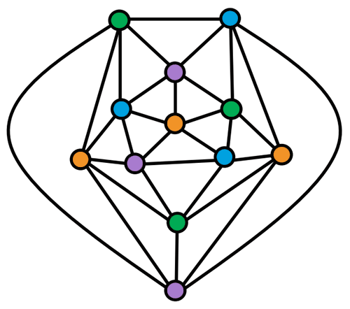
Now, a proper vertex-colouring of a graph $G$ assigns a colour to each vertex of $G$ in such a way that any two adjacent vertices have different colours. Consequently, a proper face-colouring of a map is equivalent to a proper vertex-colouring of its dual! In Figure 2, you can see a proper vertex-colouring of the dual of the dodecahedral graph.

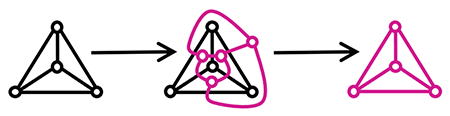
Paint-by-Number-figure-3 — Figure 3: The tetrahedral graph is its own dual.

Attentive readers may notice that taking the dual of the dodecahedral graph pleasingly produces the icosahedral graph – it transpires that the two graphs are duals of each other. These are two of the five possible Platonic graphs³: tetrahedral, cubical, octahedral, dodecahedral and icosahedral. Similar properties can be found with the other Platonic graphs: the octahedral and cubical graph are duals of each other and the tetrahedral graph is the dual to itself (see Figure 3)! Table 1 lists some properties of the five Platonic graphs, shedding light on the reasons for the emergence of this pattern.

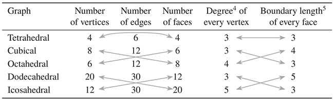
Paint-by-Number-table-1 — Table 1: Properties of the five Platonic graphs.

When we take the dual of any (finite) map, it will always generate a finite, simple⁶ and planar graph. An alternative form of the four-colour theorem now becomes apparent: given a graph $G$ that is finite, simple and planar, there exists a proper vertex-colouring of $G$ using ${\le} 4$ colours. Before we discuss the proof of the four-colour theorem, however, I would like to backtrack a little and examine the six-colour theorem.

The six-colour theorem

Throughout the following discussions of the six-colour and five-colour theorems, when I say graph, take this to always mean a finite, simple and planar graph.

For the start of this proof, we will need to use two well-known results:

(a) For any graph $G = (V,E)$ where $V$ is the set of vertices and $E$ is the set of edges, we have $\sum_{v\in V}\rd(v) = 2|E|$ where $\rd(v)$ is the degree $^4$ of vertex $v$ . (This is known as the handshaking lemma.)

(b) If $G = (V,E)$ is a simple, planar graph with $|V| \ge 3$ , then $|E| \le 3|V|-6$ .

Let us assume that there exists a graph $G = (V,E)$ such that $|V| > 6$ and the degree of every vertex in $G$ is ${\geq} 6$ . But, seeing as the degree of every vertex is ${\geq} 6$ we can state using (a) that $6|V| \le 2|E|$ , which is equivalent to $3|V| \le |E|$ . By (b), we also know that $|E| \le 3|V|-6$ , which gives us $3|V| \le |E| \le 3|V|-6$ and so we encounter a contradiction. This must mean that our original assumption was false, giving us another important result:

Next, let us pick some $k\in \mathbb{N}$ and assume that the six-colour theorem is true for all graphs with $k$ vertices. Given a graph $G'$ with $k + 1$ vertices, $G'$ must contain a vertex $v$ of degree ${\le} 5$ (see (c)). If $v$ were to be removed from $G'$ , along with its associated edges then, by our assumption, the remaining graph can be coloured with ${\le} 6$ colours. If we perform this colouring and subsequently add $v$ back into $G'$ , $v$ can be adjacent only to a maximum of 5 vertices. This means that we can always assign a colour to $v$ so that the total number of colours used by the entire graph remains ${\le} 6$ ; Figure 4 shows this in action.

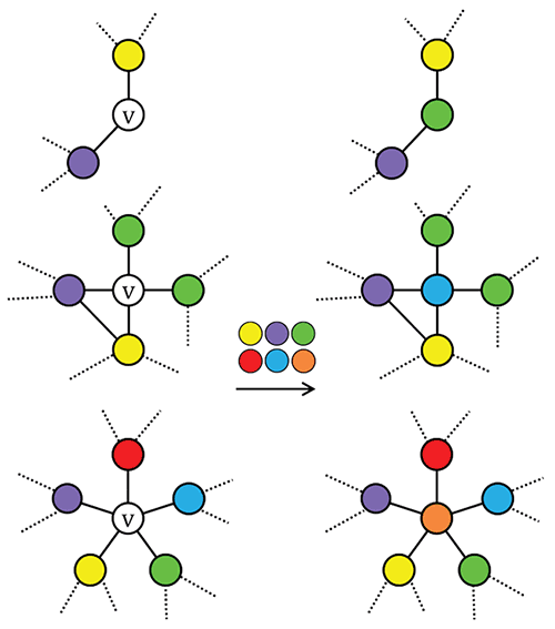
Paint-by-Number-figure-4 — Figure 4: $\bm{v}$ can always be coloured whilst keeping the total number of colours as 6 or under.

Clearly the six-colour theorem is true for all graphs with 1 vertex, hence, we have completed a proof by induction:

(d) Given a graph $G$ that is finite, simple and planar, there exists a proper vertex-colouring of $G$ using ${\le} 6$ colours.

The five-colour theorem

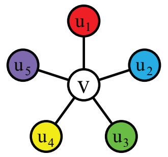Paint-by-Number-figure-5 — Figure 5: $\bm{v}$ is adjacent to 5 vertices, each of a different colour.

Can we use the same induction as we did for the six-colour theorem, for the five-colour theorem? Well, almost! The only case where this induction would break down is if, when we added $v$ back into $G$ , we found that $v$ is adjacent to 5 vertices, each of a different colour. Undoubtedly, it would be impossible to colour $v$ without using a sixth colour. Thus, if we can prove that in this case it is still possible to colour $G$ with ${\le} 5$ colours, then we will have proven the five-colour theorem.

Accordingly, let $G$ be a graph such that we have coloured $G$ without $v$ with ${\le} 5$ colours but, when returning $v$ , have found it to be adjacent to 5 vertices, each of a different colour. Label these 5 vertices $u_1, u_2, \ldots, u_5$ , as in Figure 5, and consider the following instructions:

(i) Change $u_1$ to green.

(ii) For any originally green vertex $w$ with a newly green neighbour, change $w$ to red.

(iii) For any originally red vertex $z$ with a newly red neighbour, change $z$ to green.

(iv) Repeat (ii) and (iii) until no more changes are needed.

The vertices that have changed colour now form a Kempe chain.

There are two possibilities for where this Kempe chain could travel:

(i) The chain does not reach $u_3$ – see Figure 6.
We have found a way to recolour $G$ so that $v$ no longer has 5 adjacent vertices, each of a different colour. This means that the entire graph can now be coloured with 5 colours!

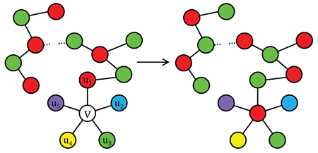
Paint-by-Number-figure-6 — Figure 6: If the Kempe chain does not reach $\bm{u_3}$ then we have successfully recoloured $\bm{G}$ with 5 colours.

(ii) The chain reaches $u_3$ – see Figure 7.
This will mean that we have recoloured $G$ but $v$ is still adjacent to 5 different colours. Fortunately, because $G$ is planar, we know that we can form a blue–yellow Kempe chain from $u_2$ that will not be able to escape the red–green Kempe chain loop. Consequently, this new Kempe chain will not be able to return to $u_4$ , the yellow vertex, and will result in a recolouring of $G$ such that $v$ is no longer adjacent to 5 different colours. A colouring of the entire graph is now possible with 5 colours!

Paint-by-Number-figure-7 — Figure 7: If the Kempe chain reaches $\bm{u_3}$ then we can form a second Kempe chain to find a colouring of $\bm{G}$ using 5 colours.

To conclude, we know that the five-colour theorem will apply to all graphs with 1 vertex. Assuming that it is true for all graphs with $k$ vertices, we can prove it to be true for all graphs with $k + 1$ vertices via the application of a Kempe chain. By induction, the five-colour theorem is true:

(e) Given a graph $G$ that is finite, simple and planar, there exists a proper vertex-colouring of $G$ using ${\le} 5$ colours.

Here is an interesting digression. Kempe chains were first described by Alfred Kempe in September 1879 within his paper titled ‘On the geographical problem of the four colours’ [1]. When this paper was published, Kempe was credited as having proven the four-colour theorem. However, 11 years later John Heawood, a mathematician at Durham University (where I am an undergraduate!), spotted a mistake in Kempe’s proof and instead realised that Kempe chains could be used to prove the five-colour theorem [2].

The four-colour theorem

Alas, our induction argument falters beyond this point, as we reach the infamous four-colour theorem. The proof of this one is significantly harder than its sister theorems and, as many mathematicians know, this theorem earned its fame because it was the first to require the use of a computer to prove it. This elicited considerable opprobrium as it was impossible for a human to confirm whether the result was correct. Sadly, the proof is too long to include within the confines of the present article but, briefly, the mathematicians Appel and Haken reduced the infinite set of possible maps to a set of only $\np{1936}$ that needed to be checked to prove that the theorem was true [3].

So, now you realise the big secret that the stationary companies do not want you to know: next time your 6-year-old is badgering you for the deluxe pen pack of 100 colours, you can bestow upon them the valuable teachings associated with the four-colour theorem and they shall, hopefully, be fully accepting of the notion that four colours will do them just fine.

Lucia P. Karageorghis
Durham University

Notes

A planar graph is one that can be drawn such that its edges only ever intersect at their endpoints.
This is not quite the usual definition, but it is good enough for our colouring purposes.
A Platonic graph is finite, simple, planar and connected with all vertices of the same degree $^4$ $d \ge 3$ and all faces of the same boundary length $^5$ $b \ge 3$ .
The degree of a vertex is the number of times that the vertex appears as an endpoint of an edge.
The boundary length of a face is the number of edges that border that face.
A simple graph is one that does not contain any loops and does not have multiple edges between two vertices.

Graham Hoare Prize 2019 winning article.

References

Kempe, A. (1879) On the geographical problem of the four colours, Am. J. Math., vol. 2, no. 3, p. 193.
Durham University (2019) Algorithms and complexity in Durham, community.dur.ac.uk/algorithms.complexity/graph.html (accessed 28 July 2019).
Rogers, L. (2011) The four colour theorem, nrich.maths.org/6291 (accessed 28 July 2019).

Reproduced from Mathematics Today, December 2019

Download the article, Paint by Number (pdf)

Image credit: Compound of 5 dodecahedra by fdecomite / Flickr / CC BY 2.0

Exploring-Steiner-Chains-with-Mobius-Transformations-featured

Exploring Steiner Chains with Möbius Transformations

Playing Tennis without Envy

Connecting the Dots with Pick's Theorem

Published 12th December 2019

Paint by Number