A Mathematician's Guide to the Perfect Mug of Tea

In ancient Chinese mythology, it is said that the god Shennong once consumed some 72 different herbs, many of which were riddled with poison. Then, Shennong drank the first tea ever produced, which flushed the toxins from his body [1]. Unfortunately, Typhoo is not exactly recognised in the medical community as a certified antidote, but it can reliably cure a hangover and it definitely makes mathematics more bearable.

In the UK alone, we drink enough tea to fill about 20 Olympic swimming pools every day. It is the first port of call any time something, however insignificant, goes wrong (or even right). We live by tea; we die by tea; we pretty much went to war with the Americans over tea. As you may be able to tell, there are few things more important to us than a good cup of tea. So, throughout this short piece, we will be exploring and exploiting some of the most universal mathematical modelling formulas in our pursuit of the perfect cuppa.

The mathematics of stuff

Before we can approach the mystic art of tea-making, we need to understand a much more general formula that governs the behaviour of pretty much any stuff you can think of. It is known by the mathematical community as the conservation of mass equation, for which Chaplain [2] provides a rather thorough algebraic breakdown. The idea is based on the fact that, fundamentally, matter can be neither created nor destroyed, so the change in density of some stuff in some place is equal to the amount of stuff coming in to said place minus the amount of stuff going out of said place.

Clearly this is not the most mathematically rigorous analysis, so let us be a bit more clever. We will be using a spatial variable $\boldsymbol{x} = (x,y,z)$ with a temporal variable $t$ , and considering an arbitrary volume $V$ , fixed in space, which is bound by a smooth, continuous surface $\partial V$ . Suppose we are investigating the evolution of some stuff, which, at position $\boldsymbol{x}$ and time $t$ , has density denoted by $\rho (\boldsymbol{x},t)$ . Here, stuff can refer to just about anything, including but not limited to chemicals, bacteria, people, disease, goats invading the Galapagos Islands, zombies, forest fires and (in our case) tea.

Under the continuum hypothesis, we may assume $\rho (\boldsymbol{x},t)$ to be a sufficiently smooth function so that, by the law of conservation of mass, the rate of change of density within $V$ is equal to the net flux of stuff across the surface $\partial V$ . We can represent this mathematically as:

$\begin{equation*} \int_{V} \frac{\partial \rho}{\partial t}(\boldsymbol{x},t) \textrm{d}{}V = \int_{\partial V} -\boldsymbol{J}(\boldsymbol{x},t) \cdot \boldsymbol{n} \textrm{d}{}S, \end{equation*}$

where $\boldsymbol{J}$ represents net flux (stuff in minus stuff out) and $\boldsymbol{n}$ is the outward pointing normal to the surface.¹ Then, by the divergence theorem, we have that

$\begin{equation*} \int_{V} \frac{\partial \rho}{\partial t}\textrm{d}{}V = \int_{V} (-\nabla \cdot \boldsymbol{J}) \textrm{d}{}V. \end{equation*}$

Since the volume $V$ was chosen arbitrarily, the integrands must be equivalent, giving the general form of the conservation of mass:

$\begin{equation*} \frac{\partial \rho}{\partial t} = -\nabla \cdot \boldsymbol{J}. \end{equation*}$

Although Chaplain’s work was based on the (arguably) more important field of cancer treatment, the principles are precisely the same for tea. What we have here is a partial differential equation, which will help us to understand exactly what is happening to both the temperature of our tea and its constituents (whether that be sugar, milk, more sugar, milk alternative, the tea itself or those crumbly bits of biscuit that break off when you are not paying attention mid-dunk).

Mixing the brew

Without diving too hastily into the minefield that is fluid dynamics, we can determine a lot about the preferred method of tea-mixing just by manipulating our equation. Let us assume (quite reasonably) that you want your tea to be evenly distributed² and you want it as soon as possible. There are only two processes that make tea³ seep out of its bag: the first is known as diffusion, which is the uncontrollable random movement of tea molecules down concentration gradients, and the second is advection, otherwise known as transport with the mixture velocity. To model this, we will need to specify an exact form for our flux vector:

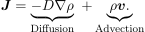
$\begin{equation*} \boldsymbol{J} = \underbrace{- D \nabla \rho}_{\text{Diffusion}} \ + \underbrace{\rho \boldsymbol{v}.}_{\text{Advection}} \end{equation*}$

Here, $D$ is known as the diffusivity coefficient, which determines the efficiency of diffusion and is usually quite small. On the other hand, $\boldsymbol{v}$ represents the velocity of our tea, which results from stirring the mixture. If we make the assumptions that flow is steady and occurs in one direction only, this allows for some massive simplifications further on. In our case, we will be stirring our tea in the ‘angular’ direction with a roughly constant velocity throughout.

The elusive Péclet number is a measure of the rate of advection to the rate of diffusion [3], and can be derived by the process of non-dimensionalisation. In general, all variables in our model have underlying dimensions, such as length per unit time (velocity) or mass per unit volume (density). Non-dimensionalisation is the process of relieving our variables of these dimensions by rescaling them with dimensionless variables and putting their dimensions into some constants. In our case, we will rewrite our variables as

$\begin{equation*} \rho = \rho_{0} \rho^{*}, \quad t = \frac{l^2}{D} t^{*}, \quad \nabla = \frac{1}{l} \nabla^{*}, \quad \boldsymbol{v} = v_{0}\boldsymbol{v}^{*}, \end{equation*}$

where $\rho_{0}$ is some constant concentration of tea, $l$ is a fixed length scale, $v_{0}$ is the magnitude of our velocity (so that $\boldsymbol{v}^{*}$ is now a unit vector), and anything with a $*$ on the end of it is a dimensionless variable.

Substituting these new variables into our conservation of mass equation yields a new, non-dimensionalised equation:

$\begin{equation*} \frac{\partial \rho^{*}}{\partial t^{*}} = -\nabla^{*} \cdot \left(-\nabla^{*} \rho^{*} + P\boldsymbol{v}^{*}\rho^{*} \right), \end{equation*}$

where $P = v_{0}l/D$ is the Péclet number. As we mentioned previously, the diffusivity coefficient is typically very small, whereas our velocity, relatively speaking, will be much larger. As such, $P$ should be very large. This means, at leading order, the advection term will dominate the diffusion term when it comes to mixing tea. So, if you want your tea to mix quickly, then it is best if you, well, mix it.

The ideal temperature

It might be a tad generous to say that the diffusion equation and the heat equation are the same; in reality, they are derived from completely different physical principles. However, as luck would have it, their functional forms are pretty much identical. We can amend our derivation of the conservation of mass equation to determine the heat equation, given as

$\begin{equation*} \frac{\partial T}{\partial t} = \alpha \nabla^{2} T, \end{equation*}$

where $T$ is the temperature (usually measured in kelvins) and $\alpha$ is the thermal diffusivity of our medium.

However, before we can apply the heat equation, we need to understand where we are applying it. Your bog-standard mug is typically cylindrical, flat-bottomed and often plastered with the words ‘World’s Best Dad’. So the best thing for us to do is convert to cylindrical polar coordinates.

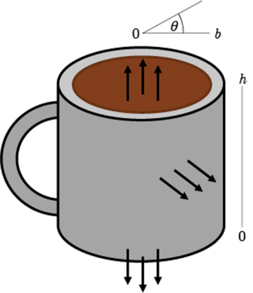
The Cylindrical Domain of a Mug of Tea — Figure 1: The cylindrical domain of a mug of tea. The arrows refer to the direction of heat flux at the boundaries.

So, we will consider a ‘cylinder’ of tea, with radius $b$ and height $h$ . Unless the tea is resting next to a radiator, there is no reason for any one side of the tea to be hotter than the other. In other words, we do not need to consider $\theta$ . Thus, we have:

$\begin{equation*} \frac{\partial T}{\partial t} = \alpha \left( \frac{1}{r} \frac{\partial}{\partial r} \left( r \frac{\partial T}{\partial r} \right) + \frac{\partial^{2} T}{\partial z^{2}} \right). \end{equation*}$

Now we need to define some conditions. When we pour our water out of the kettle, it should have roughly the same constant temperature throughout, so that initially $T(r,z,0) = T_{0}$ . In general, heat transfer across a boundary can be described by Newton’s law of cooling, which effectively states that the flux of heat is proportional to the difference in temperature between the medium and its surroundings. Let us take $T_{1}$ to be room temperature ( $T_{1} < T_{0}$ ), then we can write:

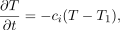
$\begin{equation*} \frac{\partial T}{\partial t} = -c_{i} (T - T_{1}), \end{equation*}$

at each of the boundaries, $r = b$ , $z = 0$ and $z = h$ . Here $c_{i}$ is the so-called cooling coefficient, which depends on the material of the boundary (such as air or ceramic). As such, $c_{i}$ will likely be different at each boundary. To complete our model, we may determine that (thankfully) the temperature at $r = 0$ should be less than infinity, or alternatively that:

$\begin{equation*} \frac{\partial T}{\partial r}(0, z, t) = 0. \end{equation*}$

This model can be solved analytically via separation of variables. We can make the boundary conditions homogeneous without altering the partial differential equation itself by using the change of variables $U = T - T_{1}$ . Then, by assuming a solution of the form $U(r,z,t) = R(r)Z(z)K(t)$ and introducing the separation constants $\lambda$ and $\sigma$ , we can reduce the problem to a system of ordinary differential equations:

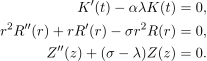
$\begin{align*} K'(t) - \alpha \lambda K(t) = 0, \\ r^{2} R''(r) + rR'(r) - \sigma r^{2} R(r) = 0, \\ Z''(z) + (\sigma - \lambda) Z(z) = 0. \end{align*}$

By applying the conditions and investigating the different values of the separation constants, we could derive a solution, but ultimately we will be left with a rather unapologetic infinite series. As such, we will not delve any deeper into the approximate solution of this exact model. Instead, we will determine an exact solution to an approximate model.

We can actually use Newton’s law of cooling to estimate the change in temperature of the entirety of the tea, without considering the spatial variation. Solving the equation as an ordinary differential equation gives:

$\begin{equation*} T(t) = T_{1} + A \textrm{e}^{-ct}, \end{equation*}$

for some constant $A$ . The initial condition $T(0) = T_{0}$ gives $A = T_{0} - T_{1}$ . It is safe to assume that the water will be boiling when we first pour it in, so that $T_{0} = 373.15\,{\textrm K}$ (temperatures here are in kelvins, so that all values are non-negative; to return to Celsius, we simply subtract $273.15$ ), and we have the heating on, so we will set $T_{1} = 293.15\,{\textrm K}$ ( $20^{\circ} \text{C}$ ). In general, the cooling coefficient of tea is quite small; an approximation of $c = 0.0005$ should suffice for most mugs. As such, the temperature of the tea at any time point $t$ will be

$\begin{equation*} T(t) = 293.15 + 80 \textrm{e}^{-0.0005t}. \end{equation*}$

Say I prefer my tea at a specific temperature $T_{2}$ and want to know how long I need to wait before I drink said tea, then I can rearrange the equation to give:

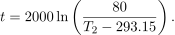
$\begin{equation*} t = 2000 \ln \left( \frac{80}{T_{2} - 293.15} \right). \end{equation*}$

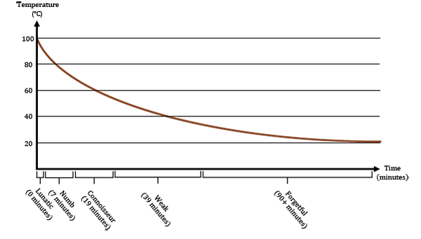
For example, I prefer my tea at a crisp $65^{\circ} \text{C}$ ( $338.15\,{\textrm K}$ ). Substituting this into our equation returns $t \approx 1150$ (seconds), which is approximately $19$ minutes. If you do not know your exact favourite temperature, I have prepared a handy chart to determine how long you should wait depending on the type of tea drinker you are — see Figure 2.

That is all from me, now go stick the kettle on.

Tea Temperature over Time — Figure 2: Tea temperature over time.

Luca Panconi
University of Birmingham

Notes

Since we are interested only in the change of concentration within the volume, we take net flux about the inward pointing normal given by $-\boldsymbol{n}$ .
In mathematical terms, we might call this a homogeneous distribution of tea.
Specifically, a mixture of amino acids and polyphenols trapped in the tea leaves.

Graham Hoare Prize 2020 winning article.

References

Christie, A. (1968) Chinese Mythology, in The Hamlyn Mythology Series, Hamlyn.
Chaplain, M.A.J. (2008) Modelling aspects of cancer growth: insight from mathematical and numerical analysis and computational simulation, in Multiscale Problems in the Life Sciences: From Microscopic to Macroscopic, Springer, Berlin and Heidelberg, pp. 147–200.
Patankar, S.V. (1980) Numerical Heat Transfer and Fluid Flow, Washington, DC, Hemisphere Publishing Corp.

Reproduced from Mathematics Today, December 2020

Download the article, A Mathematician’s Guide to the Perfect Mug of Tea (pdf)