Urban Maths: Picturing the Zeta Function

Travelling from the outskirts to the centre of town I’m bombarded with posters: in shop windows, on hoardings, on walls, even on bus shelters. The posters comprise principally pictures with just a few words, reflecting the old saying that ‘a picture is worth a thousand words’. This expression encapsulates the notion that an image can convey the essence of a complicated idea better than a detailed description. This works, not only in the world of advertising, but in mathematics as well, where complicated concepts are often illuminated by visual representations.

For example, let’s see how we might get a better feel for the Riemann zeta function through the use of some pictures rather than just the usual mathematical symbols. We’ll start with the usual symbols though!

In the first instance the zeta function, $\zeta(s)$ is defined as follows:

(1) $\begin{equation*}\zeta(s) = \sum^{\infty}_{k = 1}\frac{1}{k^s}.\end{equation*}$

Urban-Maths-Picturing-the-Zeta-Function-figure-1 — *Figure 1: Examples of $s \to \zeta(s)$ with real $s$ .*

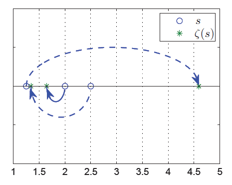
If $s$ takes the value 1, we know that the above series diverges; when $s$ is a positive even integer $\zeta(s)$ is given in general in terms of Bernoulli numbers (see [1]) and there are the well-known examples $\zeta(2) = \pi^2/6$ and $\zeta (4) = \pi^4/90$ . For $s$ as a positive odd integer greater than 1 there are no known exact expressions for $\zeta(s)$ , but it can be calculated numerically to any desired precision. The same is true for $s$ as a positive non-integer greater than 1. Pictorially, for real numbers greater than 1, we can represent $s \to \zeta(s)$ as a transition from one place to another along the real number line, as shown for three examples in Figure 1. Numbers greater than about 1.834 shrink under the transition, those less than about 1.834 get larger.

We do not need to restrict ourselves to the reals; we can also find the zeta function of complex values of $s$ (real part greater than 1) using (1). How does this work?

Urban-Maths-Picturing-the-Zeta-Function-figure-2 — *Figure 2: Trace of first 100 terms of $1.1 + 2\mathrm{i} \to \zeta(1.1 + 2\mathrm{i})$ .*

Consider a general, individual term of the series on the right-hand side of (1), and set $s = x + \mathrm{i} y$ . We can write

$\frac{1}{k^s} \to \frac{1}{k^{x + \mathrm{i} y}} \to \frac{1}{k^x} \times \frac{1}{k^{\mathrm{i} y}} \to \frac{1}{k^x} \times \mathrm{e}^{-\mathrm{i} y \ln k}.$

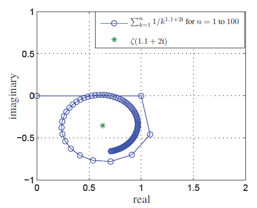
This we can think of as a vector of magnitude $1/k^x$ rotated through an angle $\theta = -y\ln k$ . The successive terms of the series in (1) add to each other vectorially, with reducing magnitudes and changing angles. Figure 2 illustrates this for the first 100 terms of $\zeta(s)$ for $s = 1.1 + 2\mathrm{i}$ . Convergence to the final value ( $\approx 0.631 - 0.353\mathrm{i}$ ) is clearly slow, and the successive terms wind round the final value many times before getting there!

Urban-Maths-Picturing-the-Zeta-Function-figure-3 — *Figure 3: Examples of $s \to \zeta(s)$ with complex $s$ .*

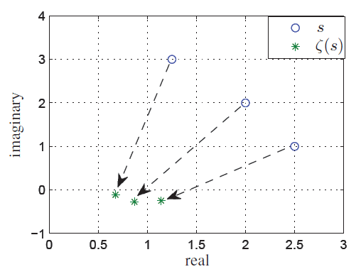
To illustrate the transition from complex $s \to \zeta(s)$ we make use of the complex plane. Figure 3 shows the transition for three example points.

Can we extend the function further to values of s whose real parts are less than 1? Well, not directly using the definition set out in (1) above as the series diverges. However, we could define a more complicated function that happened to match the definition in (1) by the following simple trick:

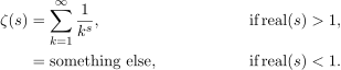
$\begin{align*}\zeta(s) &= \sum^{\infty}_{k = 1}\frac{1}{k^s}, & \text{if} & \operatorname{real}(s) > 1, \\ &= \text{something else}, & \text{if} & \operatorname{real}(s) < 1.\end{align*}$

The ‘something else’ is constructed using the concept of analytic continuation (see [2], for example). The resulting extended Riemann zeta function may be expressed as:

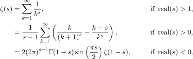
(2) $\begin{align*}\zeta(s) &=\sum^{\infty}_{k = 1}\frac{1}{k^s}, &\text{if } \operatorname{real}(s)>1, \nonumber \\&= \frac{1}{s-1}\sum^{\infty}_{k = 1}\left(\frac{k}{{(k + 1)}^s}-\frac{k-s}{k^s}\right), &\text{if } \operatorname{real}(s) > 0, \nonumber \\&= 2{(2\pi)}^{s-1}\Gamma (1-s)\sin \left(\frac{\pi s}{2}\right)\zeta (1-s), &\text{if } \operatorname{real}(s)<0,\end{align*}$

where $\Gamma$ is the gamma function (see [3], for example).

We can now create a picture of the transition $s \to \zeta(s)$ for a much greater range of values of $s$ . Instead of just three values of $s$ , let’s see what the transition looks like for a much larger number of values.

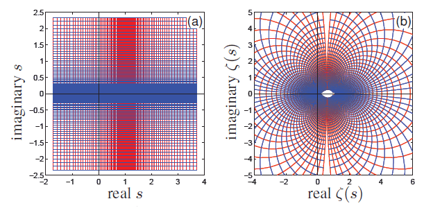Urban-Maths-Picturing-the-Zeta-Function-figure-4 — *Figure 4: Grid of (a) $s$ values and (b) corresponding $\zeta(s)$ values.*

Figure 4(a) shows vertical (red) lines, each of constant real values of $s$ , and horizontal (blue) lines, each of constant imaginary values of $s$ . Figure 4(b) shows where those lines are mapped to under the transition specified by the function definition in (2) (Note: For clarity, Figure 4(b) actually illustrates a limited, ‘zoomed in’ view, rather than showing all the transition points obtained from Figure 4(a).) In Figure 4(a) the red and blue lines clearly intersect at $90^{\circ}$ . It might not be quite so obvious, but in Figure 4(b) they also intersect at $90^{\circ}$ .

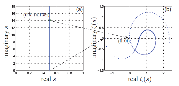
Urban-Maths-Picturing-the-Zeta-Function-figure-5 — *Figure 5: The lines (a) $s = \frac{1}{2} + \mathrm{i} y$ and (b) $\zeta (\frac{1}{2} + \mathrm{i}y)$ .*

Some values of $s$ get mapped to zero by the function defined in (2). It is clear from the inclusion of the term, $\sin (\pi s/2 )$ for example, that the function produces zero for all negative even integer values of $s$ . These are known as the ‘trivial’ zeros, but they are not the only values of $s$ that map to zero. It is known that all the other, ‘non-trivial’ zeros occur for values of $s$ where the real part of $s$ lies in the range $0<s<1$ , known as the critical strip. To date, the only known values of $s$ in the critical strip that map to zero lie on a line with real part equal to $1/2$ (the critical line). Figure 5 shows points along $s = 1/2 + \mathrm{i}y$ , where $y$ goes from 0 to 18 at intervals of 0.1, being mapped to $\zeta(s)$ . The point $s = 1/2 + 14.135\mathrm{i}$ is also included as this is the first value that maps to zero.

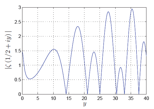
Urban-Maths-Picturing-the-Zeta-Function-figure-6 — *Figure 6: $|\zeta \left( \frac{1}{2} + \mathrm{i} y\right)|$ for $0\le y \le 40$ .*

As we travel further up the critical line we meet more zeros. Figure 6 shows the absolute magnitude of $\zeta(s)$ as $y$ goes from 0 to 40. We can see that there are six values of $s$ that map to zero in that range. In fact there are literally billions of known values of these non-trivial zeros that lie on the critical line. Riemann [4] hypothesised that the only non-trivial zeros lie along this line. This has yet to be proven (or disproven) and, if you can do it, the Clay Mathematics Institute will give you $1,000,000 [5]!

The pictures above are, of necessity given the nature of this magazine, all static. Illumination of the Riemann zeta function is even more effective with dynamic pictures. This has been done brilliantly by Grant Sanderson in a YouTube video called ‘Visualizing the Riemann zeta function and analytic continuation’ [6].

Somehow I don’t anticipate that these pictures, static or otherwise, will be adorning bus shelters any time soon!