Communicating with Convexity

Nothing takes place in the world whose meaning is not that of some maximum or minimum.
Leonhard Euler (1707–1783)

Introduction

Convexity is a fundamentally important property in optimisation. Roughly speaking, an optimisation problem is convex if its objective function is convex, as well as the set of points satifying any constraints, and in such cases the task of finding a global minimum is reduced to that of finding a local minimum. The importance of finding these minima efficiently in science and engineering applications has driven the development of software packages, such as $\texttt{cvxpy}$ from the group of Stephen Boyd at Stanford University.

Here we show that real-world problems in communications have convex formulations which can be easily implemented computationally using $\texttt{cvxpy}$ , and coded in Python. This demonstrates $\texttt{cvxpy}$ as an invaluable tool for both students and researchers in many areas of science and engineering, and has the very useful advantage that the program structure closely mirrors the mathematical description of the problem. First let us define properly what convexity means.

Convex functions

If a set $C$ is convex, then for any two points $x,y\in C$ , any point $z$ along the $x,y$ line must also be in $C$ [1, p. 23]. More formally, for $x,y\in C$ and $\theta\in [0,1]$ :

(1) $\begin{equation*} \theta x + (1-\theta)y\in C. \end{equation*}$

A function $f$ , where $f:\mathbb{R}^n \rightarrow \mathbb{R}$ , is convex if $\forall x,y\in \operatorname{dom} f$ and $0 \leq \theta \leq 1$ [1, p. 67]:

(2) $\begin{equation*} f(\theta x + (1-\theta)y) \leq \theta f(x)+(1-\theta)f(y). \end{equation*}$

This means that the function value at intermediate points of any interval is less than or equal to an affine function interpolating the end points of the interval, as shown in Figure 1. A concave function can be made convex by the operation $f\to-f$ .

Convex optimisation

A convex optimisation problem has three components:

a convex objective function $f_0(x)$ ,
$m\geq0$ convex inequality constraint functions $f_i(x)$ ,
$k\geq0$ convex equality constraint functions $g_j(x)$ ,

where $f,g: \mathbb{R}^n \rightarrow \mathbb{R}$ [1, p. 141]. We seek an optimum, $x^*\in \mathbb{R}^n$ , where $f_0(x^*)$ is a minimum. Formally the problem is defined as:

(3) $\begin{align*} &\text{minimise } && f_0(x) & \nonumber &\\ &\text{subject to } && f_i(x) \leq 0,\quad & i\in \{1,\dots,m\}\nonumber &\\ & && g_{j}(x)=0,\quad & j\in \{1,\dots,k\} &. \end{align*}$

Any local optimum $x^*$ for a convex optimisation problem is also a global optimum [1, pp. 138–139]; however, an optimum may not be unique.

Communicating-with-Convexity-figure-1 — Figure 1: The function $f(x)=x^4$ is plotted in blue. The convexity of this function can be seen by picking any two values of $x$ and noting that $f(x)$ will always lie below or on the orange chord connecting these two points.

Disciplined convex programming

In order to solve convex optimisation problems, we used $\texttt{cvxpy}$ , a symbolic programming module for Python [2] (all example code is given for Python 3). It uses a set of rules, called disciplined convex programming (DCP), to determine whether a function is convex. This is implemented using predefined classes containing functions with their curvature and sign, and using general composition theorems from convex analysis [3]. If DCP rules can be applied then interior point methods guarantee an optimal solution. The algorithm works by picking a step and direction to travel in the interior of the feasible convex set, such that the solution progresses towards optimality. For more details on barrier methods and primal-dual methods see [1, p. 561].

Example 1: water-filling

One of the simplest problems to solve in communications with convex optimisation is the classic water-filling problem. Here a total power $P$ is to be assigned to $n$ different communications channels, with the objective of maximising the total communication rate. By Shannon’s theorem [1, p. 245], an upper bound for the rate is given by $\log(1+x_i/\alpha_i)$ , where $x_i$ is the power allocated to the $i$ th channel and $\alpha_i$ is the noise power in that channel. This can be written as $\log(\alpha_i+x_i)-\log(\alpha_i)$ and the constants $\log(\alpha_i)$ are disregarded for the purposes of maximisation. Thus the communication rate, $r_i$ , of the $i$ th channel without the constant term is given by

(4) $\begin{equation*} r_i = \log(\alpha_i + x_i). \end{equation*}$

Noting that all power allocations must be non-negative, the optimisation problem can therefore be formulated as,

(5) $\begin{align*} \text{minimise} \quad -&\sum_{i=1}^{n} \log(\alpha_i + x_i) \nonumber \\ \text{subject to} \quad &x_i \geq 0, \quad \forall i \nonumber \\ &\sum_{i=1}^{n}x_i = P. \end{align*}$

This is a convex problem since $-\log(\alpha_i + x_i)$ has positive curvature within the domain $x_i \geq 0$ , and all the constraints are affine and therefore convex.

Implementation

We decided to solve the water-filling problem using $\texttt{cvxpy}$ with $n = 3$ channels and $(\alpha_1,\alpha_2,\alpha_3) = (4/5,1,6/5)$ . For simplicity we chose a dimensionless total power $P = 1$ .

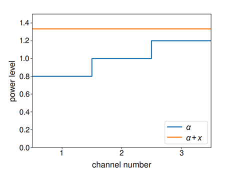
Using these parameters, the maximum communication rate is $\sum_{i = 1}^{n}r_i = 0.863$ , which is achieved with power allocations $(x_1,x_2,x_3) = (8/15,5/15,2/15)$ . This solution is shown in Figure 2, and can be seen as being analogous to filling an uneven basin to a constant level (hence the name water-filling).

Example code

To indicate the brevity of code implementation in $\texttt{cvxpy}$ we show a minimal working example below with the parameters chosen above. With an ordinary commercially available laptop, the time taken to execute the code was around 4 ms. Note that the code is a little different in formulation from the text in that it maximises $\sum_{i}^nr_i$ rather than minimising $\sum_{i}^{n}-r_i$ . The total power constraint is also rearranged to: $\sum_i^nx_i - P = 0$ .

import cvxpy as cvx
import numpy as np

n = 3 # number of channels
P = 1 # total power available to allocate
x = cvx.Variable(n) # optimisation variable x
α = cvx.Parameter(n, nonneg=True) # baseline parameter α 
α.value = [0.8,1.0,1.2]

# Define objective function
obj = cvx.Maximize(cvx.sum(cvx.log(α + x)))

# Define constraints
constraints = [x >= 0,
  cvx.sum(x) - P == 0]

# Solve problem
prob = cvx.Problem(obj, constraints)
prob.solve()
powers = np.asarray(x.value)

print('Solution status = {0}'.format(prob.status))
print('Optimal solution = {0:.3f}'.format(prob.value))
if prob.status == 'optimal':
  for j in range(n):
    print('Power {0} = {1:.3f}'.format(j,powers[j]))

Communicating-with-Convexity-figure-2 — *Figure 2: The optimal solution to the water-filling problem allocates the greatest amount of power, $x$ , to the channel with the lowest noise power, $alpha$ .*

Example 2: power minimisation in communications

To demonstrate the applicability of $\texttt{cvxpy}$ to a real-world example, we consider a system of $n$ transmitters each of power $p_k$ , ( $k=1,2,\dots,n$ ) and $m$ receivers, all in two-dimensional Euclidean space [4]. At receiver $i$ there is a power $S_i$ of the desired signal, an interference power $I_i$ from undesired signals, and a background noise $\sigma_i$ . In this problem we are constrained to having a specified minimum signal-to-interference-plus-noise ratio (SINR or $\gamma_0$ ) at each receiver, with the SINR at receiver $i$ given by,

(6) $\begin{equation*} \gamma_i =\frac{S_i}{I_i+\sigma_i}. \end{equation*}$

How can we minimise the total power consumption, $P$ , of the transmitters, yet achieve this minimum SINR, $\gamma_0$ , for all $i$ receivers ( $i = 1,2,\dots,m$ )? This question is relevant to telecom companies who want to offer a service at a minimum quality standard. We formulate the problem with a given square path-gain matrix, $G$ , background noise level vector, $\boldsymbol{\sigma} = (\sigma_1, \sigma_2, \dots, \sigma_i, \dots, \sigma_m)$ , a maximum power constraint, $P_{\text{max}}$ , of each transmitter and the fact that all transmitters must be supplied with positive power:

$\begin{align*} &\underset{p}{\text{minimise}} \quad &&\sum_k p_k\\ &\text{subject to} \quad &&p_k \leq P_{\max}\\ & \quad &&p_k \geq 0\\ & \quad &&\gamma_i \geq \gamma_0.&& \end{align*}$

Supposing that we want to receive a signal at receiver $i$ from transmitter $k$ , we define the recipient matrix, $\Delta$ , as

$\begin{align*} \Delta_{ij} = \begin{cases} 1, \quad j = k, \\ 0, \quad j\neq k, \end{cases} \end{align*}$

and our signal potential matrix $\hat{S}$ as $\hat{S} = G\Delta$ . This means that the signal received at transmitter $i$ is $S_i = \hat{S}_{ik}p_k = G_{ik}p_k$ . While the interference potential matrix is defined as $\hat{I} = G-\hat{S}$ , giving the interference at $i$ as $I_i = (\hat{I}*p)_i = \sum_{j\neq k}G_{ij}p_j$ . We must note that DCP does not allow division of the optimisation variable, $p_i$ , as it cannot guarantee curvature, so

$\begin{equation*} \gamma_i \geq \gamma_0\Longleftrightarrow \frac{S_i}{\sigma_i + I_i} = \frac{\hat{S}_{ik}p_k}{\sigma_i+(\hat{I}*p)_i} \geq \gamma_0, \quad \forall i \end{equation*}$

is rearranged to

$\begin{equation*} \hat{S}_{ik}p_k-\gamma_0(\sigma_i + (\hat{I}*p)_i)\geq 0, \quad \forall i, \end{equation*}$

which is affine, and hence a DCP function.

Path gain

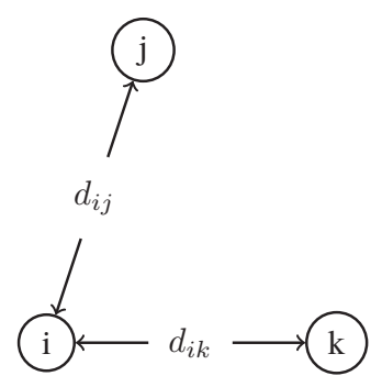
In a physical context, the path gain from transmitter $j$ to receiver $i$ , as shown in Figure 3, will depend on the distance, $d_{ij}$ , between them. Assuming isotropic propagation from each transmitter, given a pathloss coefficient, $\alpha$ , and a receiver coefficient, $A_i$ , specific to receiver $i$ , the fraction of power from $j$ that reaches $i$ is

(7) $\begin{equation*} G_{ij} = A_i/d_{ij}^\alpha. \end{equation*}$

For free space $\alpha = 2$ , while in urban environments $\alpha \sim 3.5$ [5]. Further physical complexities, such as the stochastic effects from Rayleigh fading, can easily be incorporated, whilst remaining within the DCP framework.

Communicating-with-Convexity-figure-3 — *Figure 3: Path lengths between receiver $i$ and transmitters $j$ and $k$ .*

Implementation

For ease of terminology, we will make a few simplifying assumptions. First, we set the number of transmitters equal to the number of receivers, so $n = m$ . We also pair receiver $i$ to transmitter $k$ such that $i = k$ . This means that the recipient matrix $\Delta$ is the $n\times n$ identity matrix.

All the parameters we will take as dimensionless to give simple numbers to work with. The maximum available power, $P_{\text{max}}$ , is set to $1$ . We have chosen the background noise vector, $\boldsymbol{\sigma}$ , as constant for each receiver, with $\sigma_i = 5$ . Similarly, the receiver coefficient, $A_i$ , was set to $0.025$ for each receiver.

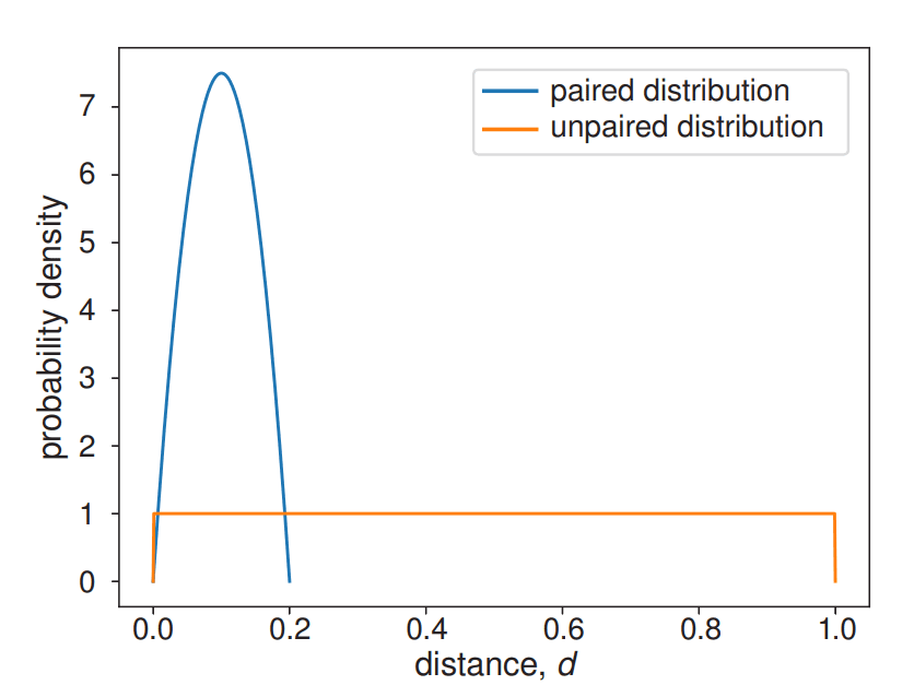
To generate the gain matrix, $G$ , we randomly sample distances from a given distribution. For paired transmitters and receivers ( $k = i$ ), we sample $d$ from a scaled $\operatorname{Beta}(2,2)$ distribution, such that $d_{ii} \sim 0.2\times\operatorname{Beta}(2,2)$ . For unpaired transmitters and receivers ( $k\neq i$ ), we sample $d$ from a uniform distribution, such that $d_{ik} \sim \operatorname{Uniform}(0,1)$ . This is illustrated in Figure 4.

Example code

For the random seed of 100 shown in the example code, the optimal total power consumption is $P = 0.381$ , with $p_1,p_2,p_3 = (0.139, 0.072, 0.169)$ . The time taken to find this solution was around 3 ms. Around 70% of the simulations with these parameters have a feasible solution, with an average optimal power consumption of $P\sim0.4$ .

import cvxpy as cvx
import numpy as np

np.random.seed(100)

# Define variables
n = 3 # number of transmitters = receivers
A = 0.025 # uniform receiver coefficient
Δ = np.identity(n) # identity matrix
# unwanted transmitters d∈U[0,1] from receivers
d_unpair = np.random.rand(n,n)
# desired transmitters d∈0.2B[2,2] from receivers
d_pair = np.random.beta(2,2,size=n)*0.20 
# make the matrix symmetric
d = np.tril(d_unpair) + np.tril(d_unpair, -1).T-np.diag(d_unpair)*Δ + d_pair*Δ

G = np.zeros((n,n)) # gain matrix G
G = A / d ** 3.5
S_hat = G * Δ # signal potential matrix
I_hat = G - S_hat # interference potential matrix

σ = 5.0 * np.ones(n)
γ = 1.0 # minimum acceptable SINR
Pmax = 1.0 # total power for each transmitter

# Define optimisation variable as the transmitter powers
p = cvx.Variable(n)

# Define objective function as the total power
obj = cvx.Minimize(cvx.sum(p))

# Define constraints
constraints = [p >= 0,
              S_hat * p - γ * (I_hat * p + σ) >= 0,
              p <= Pmax]

# Solve problem and print solution
prob = cvx.Problem(obj, constraints)
prob.solve()
powers = np.asarray(p.value)

print('Solution status = {0}'.format(prob.status))
print('Optimal solution = {0:.3f}'.format(prob.value))
if prob.status == 'optimal':
  for j in range(n):
    print('Power {0} = {1:.3f}'.format(j,powers[j]))

Outlook

Communicating-with-Convexity-figure-4 — *Figure 4: The distance between unpaired transmitters and receivers has a higher variance than paired ones, but on average the unpaired distances are expected to be greater.*

The authors hope that this article shows the utility of $\texttt{cvxpy}$ for simple ‘toy’ problems of real-world relevance. $\texttt{cvxpy}$ can handle problems with up to ${\sim} 10^3$ transmitters,
however as this takes $\sim 10^{4}$ — $10^{5}$ ms to run on a modern laptop, for very large real-world problems faster solvers and more computation power would be required. Nevertheless, one can solve convex optimisation problems with open-source software, modest computational resources and easily understood code with $\texttt{cvxpy}$ .

We believe that $\texttt{cvxpy}$ is an invaluable resource for researchers wanting to test the applicability of convex optimisation in new fields. The module could also be easily incorporated into a course on optimisation, providing students with an accessible environment to practise techniques for convex optimisation. Full code for other communication examples can be found at https://tinyurl.com/cvxpy-examples.

Robert P. Gowers
University of Warwick

Sami C. Al-Izzi AMIMA
University of Warwick

Timothy M. Pollington AMIMA
University of Warwick

Roger J.W. Hill
University of Warwick

Keith Briggs FIMA
BT Research

Acknowledgements

We would like to thank Samuel Johnson (University of Birmingham) and Steven Diamond (Stanford University) for helpful discussions, and the EPSRC and MRC for funding the University of Warwick Mathematics for Real-World Systems CDT (reference EP/L015374/1).

References

Boyd, S. and Vandenberghe, L. (2004) Convex Optimization, Cambridge University Press.
Diamond, S. and Boyd, S. (2016) CVXPY: a Python-embedded modeling language for convex optimization, Journal of Machine Learning Research, vol. 17, no. 83, pp.1–5.
Diamond, S. (2013) DCP analyzer, Stanford, dcp.stanford.edu/analyzer (accessed 18 May 2018).
Shannon, C.E. and Weaver, W. (1949) The Mathematical Theory of Communication, University of Illinois Press.
Hata, M. (1980) Empirical formula for propagation loss in land mobile radio services, IEEE Trans. Veh. Technol., vol. 29, no. 3, pp. 317–325.

Reproduced from Mathematics Today, August 2018

Download the article, Communicating with Convexity (pdf)

Set of multicoloured pencils isolated on white background © Avii | Dreamstime.com

Westward Ho! Conway, Concorde and Curiously Curved Coins

Introduction to Optimization and Hadamard…

A view across the Upper Colne Valley to Pule Hill on National Trust moorland © Andrew Hamilton | Dreamstime.com

Interview with Professor Paul Glendinning FRSE FIMA

Published 12th August 2018

Communicating with Convexity

Communicating with Convexity

Introduction

Convex functions

Convex optimisation

Disciplined convex programming

Example 1: water-filling

Implementation

Example code

Example 2: power minimisation in communications

Path gain

Implementation

Example code

Outlook

Robert P. Gowers
University of Warwick

Sami C. Al-Izzi AMIMA
University of Warwick

Timothy M. Pollington AMIMA
University of Warwick

Roger J.W. Hill
University of Warwick

Keith Briggs FIMA
BT Research

Acknowledgements

References

Related Posts

Early career mathematicians and statisticians teaching in Higher Education Ideas Exchange: Knowing the Landscape.

Academic Representatives’ Forum: Friday 21st June 2024

Presidential Address 2024

Introduction

Convex functions

Convex optimisation

Disciplined convex programming

Example 1: water-filling

Implementation

Example code

Example 2: power minimisation in communications

Path gain

Implementation

Example code

Outlook

Robert P. Gowers University of Warwick

Sami C. Al-Izzi AMIMA University of Warwick

Timothy M. Pollington AMIMA University of Warwick

Roger J.W. Hill University of Warwick

Keith Briggs FIMA BT Research

Acknowledgements

References

Related Posts

Robert P. Gowers
University of Warwick

Sami C. Al-Izzi AMIMA
University of Warwick

Timothy M. Pollington AMIMA
University of Warwick

Roger J.W. Hill
University of Warwick

Keith Briggs FIMA
BT Research