Mathematics in the Garden: Arranging Sweetcorn Plants for Maximum Pollination

I recently found an intriguing and non-trivial mathematical problem when I decided to grow sweetcorn. This plant is wind-pollinated (anemophilous), and the recommendation is to grow it in square blocks to assist pollination. Of course, as I leant on my hoe, I began to wonder whether a square block of plants really was best, particularly as the plants at the corners have only 2 close neighbours. Surely a more circular shape should be better: what was the best way to lay out the plants?

The way pollination works is that pollen from the tassels of a plant reach the silks of another, attached to the kernels of the cob. Each kernel must be pollinated, or some grey blank kernels will be produced. Achieving this is truly a gardening rather than an agricultural problem, because with a vast field of sweetcorn, pollination will be excellent. It is the gardener who wants to grow only a few plants who has problems. And gardeners short of space will grow only a handful of sweetcorn plants; my local garden centre sells young plants in packs of 8.

Clearly, a mathematical gardener would work out the optimum layout using a mathematical model of wind pollination. To make such a model, I thought of atoms in crystals, and decided that the effect $a_{ij}$ on plant $i$ of plant $j$ a distance $d_{ij}$ away should be analogous to a potential. Taking

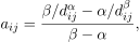
(1) $\begin{equation*} a_{ij} = \frac{\beta/d_{ij}^\alpha-\alpha/d_{ij}^\beta}{\beta-\alpha}, \end{equation*}$

where $\alpha > 0$ , $\beta > \alpha$ gives an effect that is positive (attractive) at large distances, but highly negative (repulsive) at small distances, and has a maximum value of unity at a distance of unity. Thus, this model can describe both the benefit of pollination and the disastrous effect of spacing plants too closely together. With a very large value of $\beta$ , e.g. $\beta = 40$ , optimising the layout will never cause plants to be spaced more than a tiny amount less than their optimal spacing of 1 unit (at least 1–1.5 feet for sweetcorn, depending on the variety). At distances ${>} 1$ , the repulsive term is tiny and the effect $a_{ij}$ is pollination. The inverse law $d_{ij}^{-\alpha}$ is only very slightly changed by the presence of the repulsive term.

Niklas [1] shows that the concentration $c$ of pollen a distance $d$ downwind would follow an inverse law with $c \propto d^{-\gamma}$ , where $1.75 \le \gamma \le 2$ . If $\gamma=2$ , we would need $\alpha = 3$ in (1). This is because it is not the concentration of pollen but the amount falling on the silks that determines pollination. Considering plant $i$ pollinated by plant $j$ , the angle subtended by plant $i$ is $w/d_{ij}$ , where $w$ is the plant width. Hence with a wind direction constantly changing across $360^{\circ}$ , the dose of pollen received by plant $i$ is $\propto d_{ij}^{-2} \times w/d_{ij} \propto d_{ij}^{-3}$ .

Before finding optimal planting designs, it is necessary to relate the total amount of pollen received by the $i$ th plant,

$a_i = \sum_{j \ne i} a_{ij},$

to the probability of pollination. A plausible model of the probability $p_i$ that a kernel on plant $i$ is pollinated can be derived by assuming that a unit amount of pollen received by a plant contains $N$ grains, and each grain has a tiny probability $\lambda/N$ of successfully pollinating a particular kernel. The probability that a kernel is not pollinated by any grain is $(1-\lambda/N)^{a_iN}$ , which for very large $N$ reduces to

(2) $\begin{equation*} 1-p_i = \lim_{N \rightarrow\infty}(1-\lambda/N)^{a_iN} = \exp(-\lambda a_i), \end{equation*}$

as the product-limit of the exponential function. The value of $a_i$ was found for an infinite grid of plants with unit spacing. This is over 11 times the pollen amount received from a single neighbouring plant, and must give excellent pollination. Setting pollination probability $p_{i} = 1-\exp(-\lambda a_i)$ , with $\lambda = 0.62$ , gives 99.9% pollination for an infinite field, so this value of $\lambda$ was used.

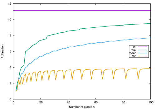
Figure 1 Mean, minimum and maximum pollinations for square plots, with an infinite plot size line — Figure 1: Mean, minimum and maximum pollinations for square plots, with an infinite plot size line

Figure 1 shows the amount of pollen received per plant against the number of plants $n$ , where plants are laid out in a square grid, with an incomplete row where necessary. The poor pollination that results from having only a few plants is clear. The minimum pollination comes from the edge plants, who have only 2 close neighbours, or 1 if a new row has just been started. For an infinite row, by the way, the amount of pollen received would be only

$2\zeta(3) = 2\sum_{i = 1}^\infty \frac{1}{i^3} \simeq 2.404,$

twice the Apéry constant.

This is the end of the mathematical modelling; from here the computer took the strain. I wrote Fortran programs that used NAG library routines, and the running times were from a fraction of a second to a few minutes on my average desktop PC. The average probability of pollination from $n$ plants,

$\overline{p} = n^{-1}\sum_{i = 1}^n p_i,$

was maximised using a NAG function minimiser that did not require derivatives to be specified, i.e. $-\overline{p}$ was minimised. Starting values were from a square grid.

Maximising the average probability of pollination means maximising the number of edible kernels produced. Other measures are, of course, possible, such as the minimax measure $\operatorname{min} p_i$ . However, with such measures, one will have fewer kernels to eat. Because $\overline{p}$ is invariant under translations and rotations, the first plant was put at $x_1 = y_1=0$ , and the second plant had $x_2 = 0$ . Imposing these constraints removes redundant parameters that can cause cycling of the iteration. The plants are indistinguishable, so with $n$ plants there must be $n!$ equivalent solutions, making the total pollination function multimodal. This did not, however, cause a problem. Many (e.g. 100) random restarts of the iteration from randomly perturbed positions were used to ensure that the function minimiser had found a maximum very close to the true one.

A colleague lives near the Cheshire Gap, where there is a prevailing wind from one direction. This can be accommodated by taking $a_{ij}$ as proportional to $\exp\{\cos \kappa (\theta_{ij}-\mu)\}$ , where $\theta_{ij}$ is the angle from the $j$ th to the $i$ th plant and $\mu$ is the angle from which the prevailing wind comes. Thus, the wind direction and variability $1/\kappa$ can be modelled, using the von Mises distribution; the results are not shown but as expected the optimal layout becomes elongated in the wind direction.

Figure 2 Placements for 4 to 7 plants — Figure 2: Placements for 4 to 7 plants

The optimum layouts with no prevailing wind are shown in Figure 2 for 4 to 7 plants. For 3 plants, the solution is to place the plants at the corners of an equilateral triangle (not shown). For 4 plants, one would perhaps expect a square layout, but instead the optimal shape is a rhombus. This means that 2 plants are closer to others and get more pollination, and the other 2 get less. To maximise the number of edible kernels of sweetcorn, 2 plants have been partially sacrificed to benefit the others and increase total pollination.

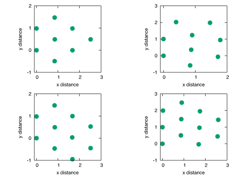
Figure 3 Placements for 8 to 11 plants — Figure 3: Placements for 8 to 11 plants

With an angle of $60^{\circ}$ , the rhombus reduces to 2 equilateral triangles pasted together. The favoured plants then have 3 near neighbours. With 5 plants, we have 2 staggered rows, and with 6 plants a pentagon with a plant in the centre. There is a big increase in pollination of 0.81 on going to 7 plants, where we have a hexagon with a central plant, compared with 0.35 on going from 5 to 6 plants, and 0.19 on going from 7 to 8 plants. Figure 3 shows the results for 8 to 11 plants, and Figure 4 shows the layout with 30 plants. It is clear that this is hexagonal planting, which is known in horticulture but seldom practised (see e.g. Jeavons [2]), with a nearly circular boundary.

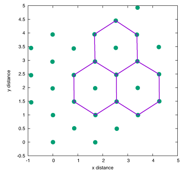
Figure 4 Placements for 30 plants showing some of the hexagons — Figure 4: Placements for 30 plants showing some of the hexagons

Hexagonal planting is optimal in general even without wind pollination, because roughly 15.5% more plants can be packed into the same area. The hexagon holds 7 plants, but each plant round the outside belongs to 3 hexagons, so we have 3 plants per hexagon; this can be seen in Figure 4. The area of each of the 6 equilateral triangles is $\sqrt{3}/4$ , giving $2/\sqrt{3} \simeq 1.155$ plants per unit area. Each internal plant now has 6 nearest neighbours, instead of the 4 found with a square grid, and edge plants have 3. The unit cell of the lattice can be taken as either a hexagon with a point in the centre or a rhombus. For large numbers of plants, the optimum placement is hexagonal planting, with some deviation at the edges to benefit edge plants.

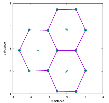
This analysis applies (pretty much) to nanoclusters, small groups of molecules on a surface. Another application of these ideas is to companion planting, where crops are interplanted with companion plants that can benefit them in several ways. For example, onions and carrots are sometimes interplanted; the carrots then help to keep away onion fly and the onions keep away carrot fly. Using mathematical modelling for optimal planting is harder, as the benefits are difficult to quantify. However, taking the same set-up as before, we have 2 types of plant, where all plants repel each other from the negative term in (1), but the first term occurs only when $j$ is a companion plant and $i$ is a crop plant. Doing this with 16 plants, of which 3 are companions, gives the elegant layout in Figure 5. This type of analysis could be useful, e.g. in planning housing developments centred on amenities, such as parks.

Figure 5 Placements for 16 plants with 3 companion plants — Figure 5: Placements for 16 plants with 3 companion plants

The mathematics here could be used to actually design optimal layouts, a practical problem being the difficulty of doing the planting, since each plant must be placed at the correct $(x,y)$ coordinates. Even hexagonal planting is harder than planting out on a square grid. A low-tech solution is to cut two bamboo poles to the required spacing. One is used to create an initial row, and then both poles are used to complete equilateral triangles and make holes for the second row, and so on. This turns out to be pretty easy.

When Voltaire had Candide say to the philosopher Pangloss ‘Il faut cultiver notre jardin’, he stressed the need to improve the world in strictly practical ways, and doubtless this included social as well as horticultural activity. Following this thought, the sweetcorn problem gives a toy model of human society. The sweetcorn plants are like individuals, some quite literally on the edge, with little social capital; these are the precariat. This is true, even though all the individuals are identical.

We can regard $a_i$ as the total wealth obtained by an individual, and $p_i$ from (2) as the utility of that wealth. Equation (2) then gives an interesting derivation of the widely used exponential utility as the probability that one’s wealth brings satisfaction, if every tiny fragment of it has a small probability of doing so. Maximising average utility $\overline{p}$ leads to some individuals having less so that others might have more and so that the average utility is larger, as in the rhombic pattern. Hence, in this model, maximising total utility leads to an unequal society, and even a minimax solution would leave some on the edge with less.

For equality, we would need plants arranged in a polygon, and with infinitely many plants, the pollination would be only $2\zeta(3)$ . However, with inequality, average pollinations of over 12 can be achieved. Even those on the edge have 3 close neighbours with hexagonal planting, giving a pollination of over 3. Hence, under the sweetcorn model of society, equality is the enemy of wealth, even for the precariat, and an unequal ordering of society gives more, even to those on the edge. This is what economists call the equity–efficiency trade-off. Arthur Okun [3] argued that policies to promote equity would lower GDP, and more than 40 years on economists are still arguing about it.

I shall leave the economists to ponder this model of society and get back to my gardening. Time to plant out those sweetcorn!

Rose Baker CMath FIMA
University of Salford

References

Niklas, K.J. (1985) The aerodynamics of wind pollination, Bot. Rev., vol. 51, pp. 328–386.
Jeavons, J. (2017) How to Grow More Vegetables, 9th edition, Ten Speed Press, California.
Okun, A. (1975) Equality and Efficiency: The Big Tradeoff, Brookings, Washington.

Reproduced from Mathematics Today, June 2020

Download the article, Mathematics in the Garden (pdf)