This paper considers the imagery generated by multiple pendula swinging from a single beam. Although it is not generally detectable, the pendulum bobs lie on a sinusoid of contracting wavelength. Instead, an onlooker sees a sequence of diverse patterns produced by the bobs. Disparity between the undetected and perceived imagery is caused by insufficient signal sampling. The sequence of visual effects is explained mathematically.
1. Introduction
Our ability to learn is, in many ways, a measure of resourcefulness. Like others, we sought the answers of our youth in the dusty basements of university libraries as all but a rite of passage. Today, the halls of knowledge are often just a mouse click away. Through video-sharing website YouTube for instance, MIT throw open their illustrious lecture theatres while fellow Americans Harvard have captivated users with truly mesmerising scientific demonstrations (e.g. a coffee mug survives a perilous fall in [1] thanks to a pencil, some string and angular momentum).
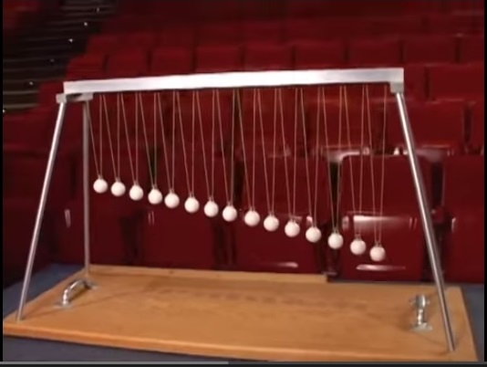
 see [2].
 In this piece we explore these effects through a mathematical model.
2. Pendulum model
Let us consider an aerial view of Harvard’s pendulum demonstration. We can describe the position of each pendulum bob by a pair of coordinates  where integral
 ![x \in [ 1, 15 ]](https://ima.org.uk/wp/wp-content/ql-cache/quicklatex.com-ed54e47338f78ecacb49da8b3efdda3d_l3.svg "Rendered by QuickLaTeX.com") denotes a pendulum’s position along a horizontal beam and
denotes a pendulum’s position along a horizontal beam and ![y \in [ -1, 1 ]](https://ima.org.uk/wp/wp-content/ql-cache/quicklatex.com-4d275448bb1bfa10877422e9fc0dfb84_l3.svg "Rendered by QuickLaTeX.com") represents a bob’s orthogonal displacement with respect to the beam (such that
represents a bob’s orthogonal displacement with respect to the beam (such that  when a bob is directly under the beam).
A simple pendulum swings back and forth under the influence of two main forces: gravity pulls the bob downwards, whilst tension in the string pulls the bob upwards. Such motion is periodic and  is sinusoidal in time [3]. Galileo showed that the simplest such wave took the form
  , where the wave has amplitude
  and frequency
  in time
  [4]. Hence we employ the following pair of equations (used by Cox in [5]) to simulate the time-evolution of Harvard’s pendula,
(1) 
(2) 
where is now a function of  and the starting position of all 15 bobs corresponds to
  (noting the addition of a
  term here).
3. Visual effects
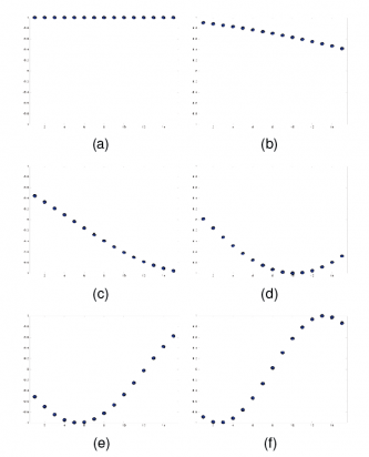
 and moments which immediately follow ((a)–(f)). A single wave appears.
 In the outset, all 15 pendula collectively form a single wave (see Figure 2). This is briefly followed by three simultaneous waves before two simultaneous waves appear in their place. Shortly afterward, three waves reappear and, as the video comes to a close, we see the gradual reappearance of a single wave. These are cyclic patterns and the video captures a full cycle.
A travelling or standing wave may be formed by any of Harvard’s pendula as they approach (and depart from) an instant when they are in phase. For example, such an instant occurs at the end of any cycle.
A cycle terminates when all 15 pendula simultaneously complete an oscillation (i.e. fall into phase). From (2), it is clear that pendulum completes an oscillation whenever  is an integer (recalling that is a function of ). Hence a cycle ends when is integral for all (i.e. for all pendula) at once. Thus,
![\[ f t = n(j) \]](https://ima.org.uk/wp/wp-content/ql-cache/quicklatex.com-640fa0ded20395dcc1a8757eeb99ed89_l3.svg "Rendered by QuickLaTeX.com")
as a cycle ends where  , the number of oscillations executed by pendulum ,
 is an integer which varies according to . Using Cox’s explicit expression for this becomes,
(3) 
where base frequency  and increment
  are -independent parameters. To be clear, any which solves (3) for all marks a cycle endpoint. Such a solution would correspond to an instant in time, i.e. unlike , would not vary according to . Therefore, these instants occur precisely when there is no explicit -dependence on the right-hand side of
(4) 
Hence must cancel out the term in the denominator of (4) at cycle endpoints. If we assume the simplest form of  can be expressed as a is a simple fraction, say
  , then
![\[ n(j) = k c \left( \frac{a}{c} + j \right) %= k c \left( \frac{b}{d} + j \right) \]](https://ima.org.uk/wp/wp-content/ql-cache/quicklatex.com-2d134d247c0cadfa8afbdee7a30705fe_l3.svg "Rendered by QuickLaTeX.com")
when a cycle ends (where  ) which gives,
![\[ t = \frac{ k c \left( \frac{a}{c} + j \right)}{ d \left( \frac{b}{d} + j \right)} = \frac{ k c \left( \frac{b}{d} + j \right)}{ d \left( \frac{b}{d} + j \right)} = \frac{k c}{d} \]](https://ima.org.uk/wp/wp-content/ql-cache/quicklatex.com-b535c07197acebf2008c3d05b449ae19_l3.svg "Rendered by QuickLaTeX.com")
in (4). It is clear that consecutive  correspond to the endpoints of a single cycle. Hence a cycle’s period,
  , equates to the difference in when is equal to, say, 0 and 1. Therefore
  and a single travelling wave appears in proximity to
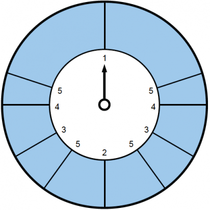
 on the clock face, every pendula are in phase (perceptible for
  in [2]). These hours are positioned according to our rule for
  .
. .
. With , we can shift our focus from endpoints to within the cycle itself. Thus we consider instants of the form
  (where
  ). Using (4), we have that
  at such instants.
 Hence, whenever :
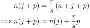
i.e.  when
when  . Put simply, this says that pendula and
  are at the same stage in their individual oscillations (while closer pendula are at different stages) when
![\[\frac{r}{s} = \frac{v}{p} \]](https://ima.org.uk/wp/wp-content/ql-cache/quicklatex.com-109e95ac39e877257ece70b578e3de63_l3.svg "Rendered by QuickLaTeX.com")
for  such that and
  are coprime. Therefore every pendula are in phase at (see Figure 3) and travelling or standing waves may form in proximity to such instants.
In summary, Cox’s model predicts and explains Harvard’s visual sequence: 1 wave near  s, 3 waves near
  s, 2 waves near
  s, 3 waves near
  s and 1 wave near
  s (
s ( s in [2]).
4. Spatial aliasing
As they exhibit simple harmonic motion, pendulum bobs can collectively produce a diverse array of imagery. Whilst predicting such variation, (1) and (2) show that Harvard’s bobs actually lie on a curve,
(5) 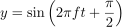
where  . That is, bobs demonstrate the ability to create multiple waveforms despite lying on a continuous sinusoid at all times (e.g. see Figure 4). This is a phenomenon known as aliasing [6] and is caused by improper sampling [7].
As pendula swing back and forth in [2], a viewer mentally interpolates between the moving bobs. Thus the spectator perceives some curve(s) of best fit, e.g. visual waves. Intuitively, all such curves would be described by (5) although this is seldom the case. Hence the ‘true’ image (as described by (5)) can go undetected by the human eye.
In short, an observer’s discrete sample (in the form of 15 pendulum bobs at equal intervals along Harvard’s beam) of the underlying curve (i.e. a continuous sinusoid) typically turns out to be an inappropriate sampling rate. Thus Harvard’s bobs do not generally provide an adequate set of data for faithful interpolation and the onlooker perceives a ‘false’ image.
False imagery of this kind (e.g. multiple waves) is unavoidable under Harvard conditions (i.e. where  ). This is because the wavelength of the underlying curve constantly shrinks (see (5)) [6] and therefore a viewer’s sampling rate continually falls. Hence the same sample that initially captures the underlying curve becomes unsuitable and aliasing is inevitable.
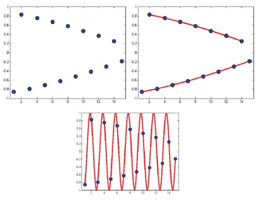
 , simulated using Cox’s model (left) with perceived waves highlighted (right) and underlying curve (centre).
5. Discussion
We have highlighted an example of behaviour that is complicated but not complex [8]. In [2] Harvard demonstrate that, without influencing each other’s motion, oscillating objects can generate imagery suggestive of coordination. Here, a mathematical rule that does not describe all such imagery is used to predict it.
Gaps between pendula (or, more generally, data points) can transform our perception of a curve or pattern. While generally undesirable, masquerading of signals creates mesmeric optical illusions in [2]. In this way, aliasing can enrich the visual effects of objects in motion. A simple deterministic rule can thus produce diverse spatio-temporal behaviour.
Andrew D. Irving
University of Liverpool
Ebrahim L. Patel
University of Oxford
Notes
- We encourage readers to watch [2] as description alone cannot do it full justice.
- Photo courtesy of Harvard Natural Sciences Lecture Demonstrations, FAS Science Division. We would like to thank Allen Crockett for granting us permission to use this image.
- This simulation uses Cox’s model with
 , i.e. such that the leftmost pendulum is longest in each picture.
 - Strictly speaking, a standing wave pattern is not a wave. This kind of pattern results when two or more waves of equal frequency travel in different directions such that they cause interference [9].
- Two pendula are in phase here if they occupy the same position (i.e. equally displaced from their initial setting) and exhibit the same behaviour (i.e. going in the same direction). As such, two pendula are in phase when they are at the same stage in their oscillations.
- By definition, a pendulum’s frequency is equal to the number of oscillations that occur per unit time [10]. Hence
 is equal to the number of oscillations executed. Therefore is also equal to the number of oscillations (made by pendulum ).
 - Cox uses d to denote the ‘incremental frequency’ of the pendula (i.e. the change in frequency with x) and b to denote the ‘base frequency’ (i.e. the frequency in the absence of any incremental change).
- Over the course of Harvard’s cycle, each pendulum completes one oscillation more than the next shortest pendulum [11], i.e.
 when
when  . Hence,

in Harvard’s case (which means that
divides and that  ).
). - The denominator on the right-hand side of (4) is the frequency of pendulum (and this does not vary according to time). Therefore, dividing time (i.e. the left-hand side of (4)) in the manner we have corresponds to dividing only the numerator of the right-hand side.
- This rule does not apply unless
 .
. - By simulating Cox’s model slowly (using Matlab for example), we can also briefly see four simultaneous waves near
 and
and  although these are difficult to perceive in [2].
 - Simple harmonic motion is a good approximation to the motion of a simple pendulum [12].
Acknowledgement
Andrew Irving would like to express his deep gratitude to the University of Liverpool for allowing him to carry out his share of this work from within their Maths Department (with special thanks to Peter Giblin, Stephen Downing and Rachel Bearon for their kindness).
References
- Harvard Natural Sciences Lecture Demonstrations (2011) Coffee Mug on String, www.youtube.com/watch?v=RMWJ7wA09gE (accessed 3 June 2014).
- Harvard Natural Sciences Lecture Demonstrations (2010) Pendulum Waves, www.youtube.com/watch?v=yVkdfJ9PkRQ (accessed 28 April 2014).
- The Physics Classroom (2014) Pendulum Motion, www.physicsclassroom.com/class/waves/Lesson-0/Pendulum-Motion (accessed 28 April 2014).
- Budd, C. (2013) Maths makes waves!, http://people.bath.ac.uk/mascjb/PUSArticles/Waves.pdf (accessed 1 July 2014).
- Cox, E. (2012) Pendulum Wave Demonstration With Matlab, http://ericboy.wordpress.com/2012/05/20/194/ (accessed 28 April 2014).
- Flaten, J.A. and Parendo K.A. (2001) Pendulum waves: A lesson in aliasing, Am. J. Phys., vol. 69, no. 7, pp. 778–782.
- Olshausen, B.A. (2000) Aliasing, http://redwood.berkeley.edu/bruno/npb261/aliasing.pdf (accessed: 9 May 2014).
- IMA Public Lectures (2014) Making Sense of a Complex World, www.youtube.com/watch?v=q_n1hKQIuIU (accessed 13 July 2014).
- The Physics Classroom (2014) Formation of Standing Waves, www.physicsclassroom.com/Class/waves/u10l4b.cfm (accessed 27 May 2014).
- Parks, J.E. (2000) The Simple Pendulum, www.phys.utk.edu/labs/simplependulum.pdf (accessed 10 May 2014).
- Harvard Natural Sciences Lecture Demonstrations (2014) Simple Harmonic (and non-harmonic) Motion, http://tinyurl.com/HNSLD (accessed 28 April 2014).
- Butterworth, J. (2014) Simple harmonic motion: the swing of the pendulum, The Guardian, http://tinyurl.com/shm2014 (accessed 23 May 2014).
Reproduced from Mathematics Today, December 2014
Download the article, Pendulum Pattern Perception (pdf)