Modelling Road Accidents

1 Introduction

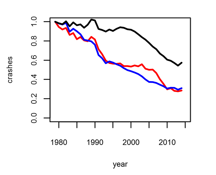
Road accidents are, fortunately, rare events. They occur randomly but on a systematic background in space and time: that is, they generally occur more frequently at locations, and at times, when there is most traffic. If you were to produce a scatterplot of accident locations in any region of the country you would broadly observe that the main road network was traced out, with clusters of accidents along busy stretches of road and around busy intersections. The annual numbers of collisions on Britain’s roads has reduced by 43% over the period from 1979 to 2015, as may be seen in Figure 1, and fatal and serious collisions by around 70%, even though vehicle mileage has been increasing by on average around 1% per year.

modelling-road-accidents-figure-1 — *Figure 1: Index of annual fatal (red), serious (blue) and total (black) collisions (1979–2014)*

Despite this generally encouraging trend, road safety is still an important issue and one that can easily generate fierce debate and controversy! It is also an area where the application of mathematics and statistics can play a vital role in shedding light on (and hopefully influencing) central and local government policy and practice.

Let us just ponder for a moment some of the questions that may naturally arise in the consideration of road safety, and that government or other agencies may need to address. How does the UK compare in road safety with other countries, and how should such comparisons be carried out, allowing for the differences in countries’ populations, numbers of registered vehicles, and extent of road network? What would be the likely effect of a graduated licensing scheme (e.g. increasing the minimum age at which a person can hold a driving licence and/or placing restrictions on the times of day they can drive or the passengers they may carry in the first year of having a licence)? What is the likely effect of changing speed limits on UK roads (as happened in April 2015 when HGV speed limits were raised from 40 mph to 50 mph on single carriageway roads and from 50 mph to 60 mph on dual carriageways)? Do speed cameras reduce accidents? What differences are there in accident risk for drivers of different ages and genders and, if a fair car insurance premium were to be deter-mined by a function of driver age, gender, and mileage driven, as well as the type of car, what would that function look like? How well is it possible to predict the number of accidents on a stretch of road, knowing the type of road, the traffic flow it carries and its design or geometry? Are there some makes and models of car that are inherently less safe than others? Some of these questions will be addressed in this article which is intended to give a flavour of some of the statistical modelling work that is carried out in the field of road safety.

But before moving on to descriptions of these modelling topics, something should be said about the data that are used in the modelling. Police attending the scene of a road accident in the UK are required to record the details of the accident when it has resulted in the injury of any one of the people involved in it. These details are then entered into what is known as the STATS19 system, and comprise information such as the date, time, location (as a grid reference), severity, vehicles involved, lighting and road surface conditions and many other factors relating to the collision. In 2015 there were just over 146,000 such collisions of which 1,658 involved a fatality. The data are available for download at data.gov.uk/dataset/road-accidents-safety-data as csv files, and hence it is relatively straightforward to determine the number of collisions at any specified site (e.g. length of road) over any specified period.

2 Predictive accident modelling

In the 1980s, the Transport Research Laboratory (TRL) carried out a series of studies for the UK Department for Transport on accidents at various types of sites: for example, four-arm roundabouts, four-arm urban signalised junctions, mini roundabouts and rural single carriageway links, to name just a few. The purpose was to investigate how the number of accidents at a site was affected by the flows passing through the site and the geometry or design of the site, with the idea of being able to see what features of design made some sites safer than others so that these findings could be embodied in design manuals. Once the accident, flow and design data had been collected for a sample of sites, generalised linear modelling (GLM) was applied to develop the models. The models ranged from the highly aggregate, relating the total number of accidents per year to some measure of the total flow passing through the site, to the rather disaggregate, providing models for each of the various types of collision. An example of the former is shown in (1) for three-arm priority junctions:

(1) $\begin{equation*}\lambda_\text{total} = 0.19{QN}^{0.53}\end{equation*}$

where QN is the encounter products flow function. The more detailed disaggregate models were fitted to the different types of collisions, relating them to the relevant flows and design features for each arm of the junction. As an example, the expected number of principal right turn collisions at four-arm signals is given by the model in (2):

(2) $\begin{equation*}\lambda_\text{prin-rt} = 0.179 Q^{0.59}_1 Q^{0.48}_2 K_1 K_2 K_3 K_4\end{equation*}$

where Q₁ is the right-turning flow on an arm and Q₂ is the straight-ahead flow on the opposing arm, and the factors following are functions of various aspects of the design of the junction involving inter alia the angle between the arms, the staging structure of the signals, and whether there is a central island. The paper by Maher and Summersgill [1] dealt with many of the methodological issues that arose in this long series of studies. The models are, of course, far from perfect in that there will always be other variables, not included in the fitted model, that have an effect on the accident rate. So although it is believed that the number of accidents at any site is Poisson distributed, the mean of this Poisson is only partly explained by the flow and design variables, and so the dependent variable is assumed to be negative binomially distributed: that is, a Poisson variable about a mean that is gamma distributed. The gamma distribution then models what is known as the overdispersion. There is no particular reason, other than mathematical convenience, why a gamma should be assumed – but the outcomes do not seem to be unduly sensitive to the choice of form of overdispersion distribution. Typically the precision of these models is such that the predicted means have a coefficient of variation of the order of 0.3.

One of the possible uses of predictive accident models is in blackspot identification: selecting which sites in a local authority’s network should be considered for remedial treatment. Instead of simply choosing the sites that have had the highest number of accidents in the last few years, it should be more efficient to choose those that have the greatest excess of accidents over the number predicted by the model for that type of site carrying that amount of traffic. Another use is in Bayesian estimation of the true mean accident rate at a site: given an observed number of accidents at a site, you should take a weighted average of that and the number predicted by the model, with weights that take account of the precision of the model.

3 Do speed cameras effectively reduce accidents?

There are few topics in road safety that generate as much heated debate as the effectiveness of speed cameras! First introduced in the early 1990s, there are now many thousands of camera sites across the UK. Whether they are there to simply make money in speeding fines or to save lives and reduce collisions is the big controversy. Because of the controversy the UK Department for Transport commissioned, in 2001, a study to evaluate the national safety camera programme but even the publication of the report on this [2] did little to stem the arguments.

The main problem in the before-after analysis of data from speed camera sites is that sites are typically selected for treatment because of a high accident number in the preceding three years. Because of the random nature of accident frequencies, the accident rate in this period is not a reliable reflection of the true before rate. This is due to bias by selection and generally, after selection, the accident rate will fall due to regression to the mean (RTM) – even if no treatment is applied! This has been well documented but unfortunately still poorly understood by many road safety professionals. So one finds claims made by local authorities that the observed reductions in numbers of accidents at camera sites are solely due to the effectiveness of cameras, when it is clear that they have made no allowance for RTM, or even for trend (as in the Transport for London (TfL) press release in September 2014 [3], which attributed the 58% reduction in fatal and serious collisions to the cameras). An idealised form of the profile of accident rate over time at camera sites is shown in Figure 2.

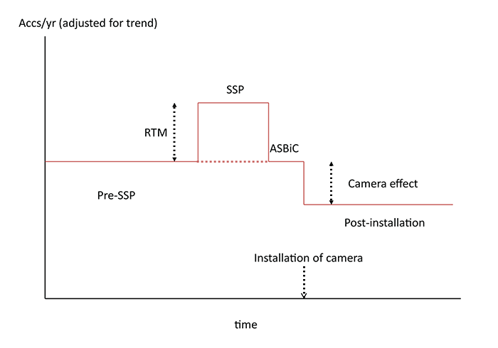
modelling-road-accidents-figure-2 — *Figure 2: Idealised form of plot of crashes per unit time, adjusted for trend*

Relative to the rate in the before period, the level is raised during the site selection period (SSP), and then falls back to its original level in the period after selection but before the installation of the camera (the ASBIC period). After installation, the level reduces further – if the cameras are effective in reducing collisions.

In principle, the course of action for analysis is quite clear: we should compare the rate of accidents after installation with that prevailing before the SSP, so as to avoid the problem of RTM. If we do not, the estimate of the effectiveness of the cameras is likely to be exaggerated. Unfortunately in practice this is not straightforward because local authorities, for some reason, do not routinely record the period used for site selection and sometimes there is an appreciable period between the decision to install a camera and the installation itself, and this period may be different for different camera sites. Therefore it is not possible to say for sure how far back we need to go to avoid including the SSP in the before period. However it is possible with some inspection and analysis of the data to make a reasonable estimate of the likely range of the SSPs.

The model we assume is

(3) $\begin{equation*}E(y_{it}) = k_i R_t F_d\end{equation*}$

where $E(y_{it})$ is the expected number of collisions at site $i$ in year $t$ , $R_t$ is the regional total of collisions in year $t$ (to allow for a trend), and $F_d$ is a factor to allow for the year $t$ relative to the year of installation $s(i)$ of the camera at site $i$ , so that $d = t - s(i)$ . If a negative binomial model is then fitted, we can estimate how the factor $F$ depends on $d$ and use this to get an idea of the range of SSPs.

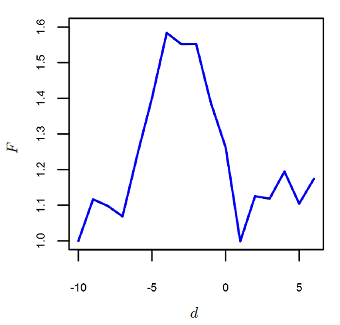
modelling-road-accidents-figure-3 — *Figure 3: Estimated profile of factor F showing raised level of fatal and serious collisions*

Fitting this model to the 497 fixed camera sites installed in London between 1992 and 2009, using the annual accident data available on the TfL website [4], the graph of $F$ against $d$ is shown in Figure 3. Whilst far from the clean idealised form of Figure 2, it is possible to see the expected raised level in the years prior to installation $(d < 0)$ and stretching back to six years before installation. This indicates that it is necessary, in order to avoid the problem of RTM, to obtain the estimate of the camera effect by comparing the collision rate after installation $(d > 0)$ with that over the years that are at least six years before installation $(d \le -6)$ .

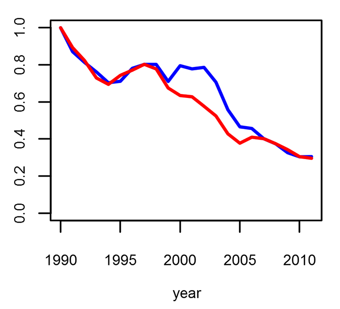
When this is done, it is found that there is no evidence of any significant reduction in fatal and serious collisions at the camera sites, contrary to the claim made in the TfL press release of September 2014 [3]. This is confirmed visually in Figure 4, in which the performance of the camera sites only matches that of all other sites in the decline in fatal and serious collisions over a 20-year period. Further details of the modelling can be found in Maher [5].

modelling-road-accidents-figure-4 — Figure 4: Indices of annual numbers of fatal and serious collisions at camera sites (blue) and non-camera sites (red)

Although there is no discernible reduction in numbers of collisions in London, it should be pointed out that some studies have shown some significant benefits from the installation of cameras. The study commissioned by the RAC Foundation [6] analysed data from ten camera partnerships (covering in total 553 cameras) and found average reductions of around 14% in Personal Injury Collisions (PICs) and 22% in fatal and serious collisions after allowance for trend and RTM. There is currently something of a gradual move away from spot speed cameras towards average speed cameras (which use number plate recognition technology to measure the average speed of vehicles over a length of road), and again the RAC Foundation has commissioned a study [7] on the analysis of collision data from all current UK average speed camera sites.

4 Modelling of two-car crashes

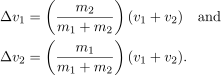
Vehicle mass is known to be a key variable in the safety performance of a vehicle in a crash. In a two-car crash, the injury risk to the occupants of the lighter car tends to be higher than that of the heavier car due to the greater velocity change in the collision. In the case of a frontal collision between vehicles of masses $m_1$ and $m_2$ travelling with speeds $v_1$ and $v_2$ , simple Newtonian mechanics show that the velocity changes of the two vehicles are:

(4) $\begin{equation*} \begin{split} \Delta v_1 &= \left (\frac{m_2}{m_1 + m_2}\right )(v_1 + v_2) \quad \text{and} \\ \Delta v_2 &= \left (\frac{m_1}{m_1 + m_2}\right )(v_1 + v_2). \\ \end{split} \end{equation*}$

In a study of 2,485 two-car frontal collisions in which at least one of the drivers was killed or seriously injured [8], the objective was to establish how the probability of injury for each driver depended, via a logistic function, on the ratio of the masses of the two cars as well as their sizes (length $\times$ width, in $m^2$ ) and the age and gender of the driver. The data set was compiled from STATS19, the vehicle registration numbers, and the make and model of the cars, with their masses and sizes obtained from a UK car magazine. The complicating features of the modelling were (i) to take account of the conditional joint injury probabilities due to the lack of data for cases where no driver is injured, and (ii) the lack of data on vehicle speeds at impact, so that a distribution for the common closing speed was assumed (with separate distributions for the known speed limit at the site of the crash) with parameters that were estimated in the model fitting process.

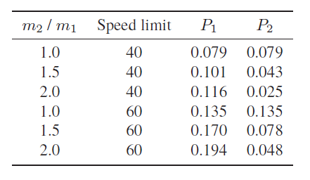
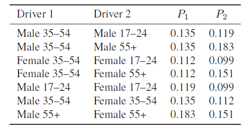
modelling-road-accidents-table-1 — *Table 1: How injury probabilities depend on mass ratio and speed limit*

Table 1 shows some examples of the results for the injury probabilities for the reference category where both drivers are males aged 35-54. It can be seen clearly how the ratio of injury risk probabilities for the two drivers varies as the mass ratio varies, with the lighter vehicle driver suffering a greater risk of injury as the mass of his/her car decreases relative to that of the other car. Vehicle size was found have a protective effect on the occupants of that vehicle. Table 2 then shows the effect of age and gender of the drivers, for the case of cars of equal mass, and in a 60 mph speed limit. It can be seen that female drivers have a lower injury risk than male drivers of the same age. This is contrary to the prevailing belief that male drivers are less vulnerable to injury due to their greater physical strength. One possible explanation for this finding is that the types of car driven by female drivers are different to those driven by males. For example, they may drive newer cars or models that have better secondary features. However, the finding about the effect of age (that is, that younger drivers have a smaller injury risk than older ones, all other factors being equal) is in accordance with prevailing wisdom.

modelling-road-accidents-table-2 — *Table 2: How injury probabilities depend on age and gender*

The same methodology was applied to other types of two-car collisions: front to side and front to back. Broadly similar findings were obtained with regard to the effect of age and gender. The protective effect of size over and above the effect of mass found for the head-on collisions was also found in front to side collisions, but was absent in front to back collisions.

5 Conclusion

The article has aimed to give some small insight into areas of road safety research where statistical modelling can play an important role in informing and influencing practice and policy in local and central government. Finally, returning to a couple of the questions raised in the introduction to this article, the government has been dragging its feet on bringing forward proposals for a graduated licensing scheme, despite a TRL study having estimated that such a scheme would save over 4,400 casualties and £224 million annually. The interested reader is referred to a RAC Foundation blog on the topic [9]. And on the topic of fair motor insurance premiums, it should be noted that a European Court of Justice ruling in 2012 made it illegal for insurance firms to take gender into account when calculating premiums. However, they are allowed to take note of age and profession so, for professions where there is a pronounced gender imbalance (for example, civil engineering or nursing), there may be an indirect effect of gender in the determination of premiums. The whole topic of how insurance premiums are calculated is discussed in some detail in an article by Birkenhead [10] in Mathematics Today.

Mike Maher FIMA
University College London

References

Maher, M. and Summersgill, I. (1996) A comprehensive methodology for the fitting of predictive accident models, Accid. Anal. Prev., vol. 28, no. 3, pp. 281–296.
Gains, A., Nordstrom, M., Heydecker, B., Shrewsbury, J., Mountain, L. and Maher M. (2005) The National Safety Camera Programme: Four-year Evaluation Report, Department for Transport.
Transport for London: press release (September 2014) tfl.gov.uk/info-for/media/press-releases/2014/september/tfl-upgrades-london-s-safety-cameras
London speed camera collision data, data.london.gov.uk/dataset/safety-camera-data-london
Maher, M. (2015) A note on the modelling of TfL speed camera data, iris.ucl.ac.uk/iris/browse/profile?upi=MJMAH36.
Allsop, R.E. (2013) Guidance on Use of Speed Camera Transparency Data, RAC Foundation.
Owen R., Ursachi G. and Allsop R. (2016) The effectiveness of average speed cameras in Great Britain, RAC Foundation (to be published in autumn 2016).
Tolouei, R., Maher, M. and Titheridge, H. (2013) Vehicle mass and injury risk in two-car crashes: a novel methodology, Accid. Anal. Prev., vol. 50, pp. 155–166.
RAC Foundation (2014) Young driver safety: why are we still not considering graduated licensing? https://racfoundation.wordpress.com/2014/11/17/young-driver-safety-why-are-we-still-not-considering-graduated-licensing/
Birkenhead, J. (2015) Are you paying too much for your car insurance? Math. Today, vol. 51, no. 1, pp. 20–23.