A Diagrammatic Construction of Indefinite Integrals: Confronting the Elusive +C

Multiple representations of mathematical concepts reveal different aspects of their properties. Constructing links between pictorial and algebraic representations allows for deeper understanding and is therefore a powerful tool to extend learning in the mathematics classroom. The interpretation of definite integrals as the area under the curve is common practice but indefinite integrals are usually approached using algebra only. This article examines a series of learning activities around the gradient function from my Year 12 Curve Sketching Summer School at UCL. Their ultimate aim is to lay down the path to constructing a diagrammatic representation of indefinite integrals. No equations are used in the activities throughout except when clearly stated. Firstly the gradient function is explored as a purely geometrical feature of a curve by using computer animations and students are then asked to sketch the corresponding gradient function of given curves. Bringing this idea to the familiar territory of quadratics and cubics, students are given a card matching activity where they need to match graphs to their corresponding gradient function and vice versa. Finally students are presented with three different quadratic graphs drawn on blank coordinate axes and requested to sketch the cubic whose gradient function corresponds to the given quadratics. The outcome is a diagrammatic construction of indefinite integrals and an insight into the elusive integration constant, $+C$ . This task also provides the classification of cubics according to the number of stationary points. These activities are usually well received by the students with feedback along the line of ‘we get the $+C$ now.’

Introduction

The ability to tackle problems using a variety of strategies is an essential problem-solving skill but it is striking how lacking our students’ mathematical toolkit is. Algebra is the beginning and the end of their problem-solving strategies. The first step to develop problem-solving power is therefore to add a few more tools to our toolkit and diagrams are a great place to start.

Multiple representations of mathematical objects reveal different aspects of their properties. Constructing links between diagrammatic and algebraic representations allows for deeper understanding and is therefore a powerful approach to extend learning in the mathematics classroom. Calculus is a particularly suitable topic for exploring those links. Pictorial representation of the gradient function and the interpretation of definite integrals as the area under the curve are common practices. By contrast indefinite integrals are usually approached using algebra only. This article describes a series of learning activities designed to explore a diagrammatic representation of the gradient function which leads to the construction of a diagrammatic representation of indefinite integrals.

1. The gradient function

Given that integration is the inverse operation of differentiation, establishing a pictorial approach to differentiation is a sensible first step towards a diagrammatic representation of indefinite integrals. This journey therefore begins with the examination of the gradient function as a purely geometrical feature of a curve.

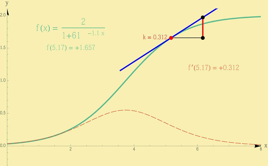
The activities involved exploring the instantaneous rate of change for polynomial functions of degree $2$ , $3$ , and $4$ (the software used was Wolfram Demonstrations Project, Instantaneous Rate of Change: Exploring More Functions with the First and Second Derivatives [1]). Figure 1 shows the example of the quadratic function. The demonstration allows the user to move the tangent along the curve by means of a slider that changes the $x$ -coordinate of the point of contact of the tangent and the curve. The gradient of the tangent is shown as $k$ in a right-angled triangle drawn from the point of contact. The horizontal side of the triangle has fixed length $1$ as the tangent slides along the curve so that the length of the vertical side is equal to the gradient of the tangent. Note that the coordinate axes are not drawn in equal aspect.

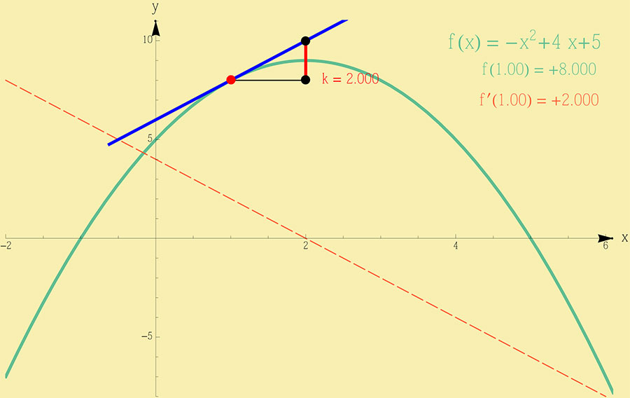A-Diagrammatic-Construction-of-Indefinite-Integrals-Confronting-the-Elusive-C-figure-1 — *Figure 1: A quadratic function with a tangent and its gradient $k$ . The corresponding gradient function is a dashed line.*

The aim of the first activity was to record the gradient at each and every point of the function and draw a curve that represents what we refer to as the gradient function. This is, of course, not possible but we can observe how the gradient of the tangent behaves and have an educated guess at what the gradient function looks like. The curve can be regarded as an object and, by sliding the tangent along the curve, we can ‘see’ the changing gradient. This image provides ‘a sensible approach’ to differentiation, based on our human perceptions [2]. The intervals where the gradient is positive, negative or zero, can then be easily determined. ‘Surfing’ the curve might be a novelty to some students but generally they can quickly make sense of it. By drawing from the students’ prior knowledge of differentiation, the conclusion that the gradient function is a straight line with negative gradient, crossing the $x$ -axis at $x = 2$ , is inevitably reached. Figure 1 shows both the quadratic function and its corresponding gradient function (dashed line). The demonstration offers the option to plot both the first and the second derivatives of the function.

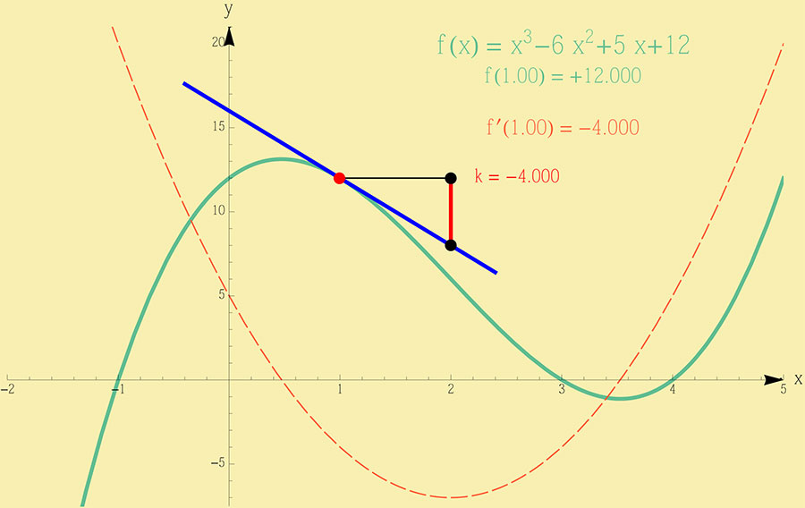
Once the pictorial representation of the gradient function has been introduced, we need to establish some strategies that allow us to sketch the gradient function in a more systematic way. By starting with the values of $x$ where the gradient is zero, the roots of the gradient function can be determined. Next we identify the intervals where the gradient is positive and where the gradient is negative. Using a cubic function with two stationary points as our next example, prior knowledge informs the students that the gradient function is a quadratic and the problem is therefore reduced to finding a quadratic that fits the requirements. Students can usually do that successfully. Figure 2(a) shows the cubic function with its corresponding gradient function.

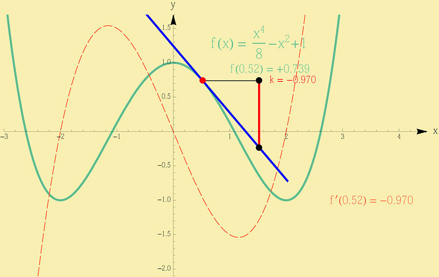
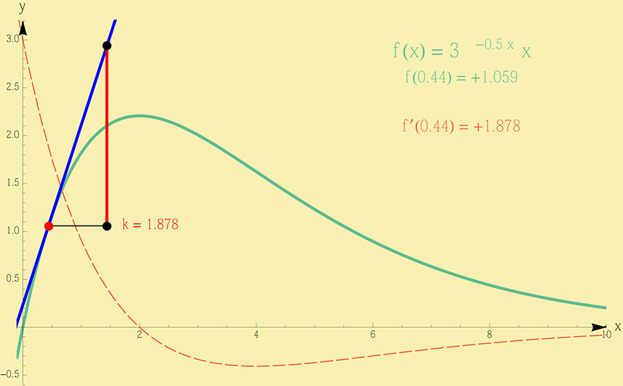
The students are then given a worksheet with three more curves, namely a quartic with three stationary points, an exponential, and a logistic function, as shown in Figure 2 together with their corresponding gradient functions. These are more challenging than the previous two functions.

The quartic function acts as a consolidation exercise since the strategies established with the cubic function can be directly applied here. The exponential function adds a new challenge with the horizontal asymptote as $x \rightarrow \infty$ but still offers all the expected features, i.e. an interval of increase leading to a point where the gradient is zero, followed by an interval of decrease. Negotiating the horizontal asymptote is done fairly successfully, especially if students are working in groups, but some clarification might be needed. The logistic function is the most challenging. This is a strictly increasing function with no stationary points, a point of inflection and a horizontal asymptote, therefore following the method used so far is of little help. Students should be nudged to observe that, since the function is strictly increasing, the gradient function is above the $x$ -axis. Some students are able to come up with the bell-like shape of the gradient function but few align its point of maximum with the point of inflection of the logistic function.

A-Diagrammatic-Construction-of-Indefinite-Integrals-Confronting-the-Elusive-C-figure-2a — *(a)*

A-Diagrammatic-Construction-of-Indefinite-Integrals-Confronting-the-Elusive-C-figure-2b — *(b)*

A-Diagrammatic-Construction-of-Indefinite-Integrals-Confronting-the-Elusive-C-figure-2c — *(c)*

A-Diagrammatic-Construction-of-Indefinite-Integrals-Confronting-the-Elusive-C-figure-2d — *(d) Figure 2: (a) A cubic, (b) a quartic, (c) an exponential and (d) a logistic function, and their corresponding gradient functions (dashed line).*

2. The derivative puzzle

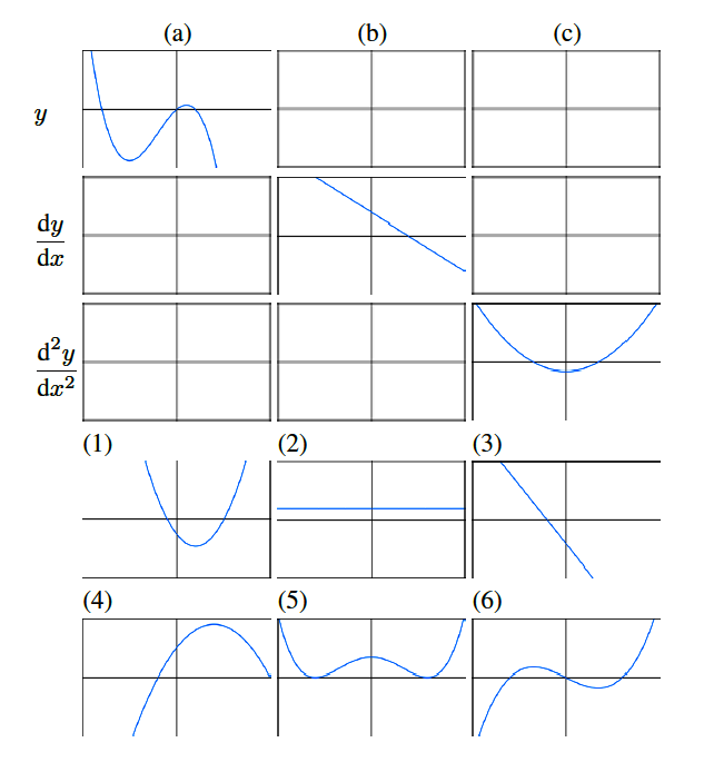
A-Diagrammatic-Construction-of-Indefinite-Integrals-Figure-3 — Figure 3: The derivative puzzle’s goal is to place the six given graphs labelled (1) to (6) on the grid so that when you work down each column the first derivative is below each graph. Graphs (1) and (2) are upside down.

Bringing this concept to the familiar territory of quadratics and cubics, students are given a matching activity where they need to match curves to their corresponding gradient function and vice-versa. Nine graphs are to be arranged in a $3$ by $3$ grid so that three functions are placed in the first row, and their corresponding first and second derivatives in the second and third rows respectively. The grid comes with three graphs pre-loaded in the leading diagonal and the other six graphs are given in separate cards. Figure 3 shows the derivative puzzle grid and the six graph cards labelled ( $1$ ) to $(6)$ .

Filling in column (a) is merely an exercise in finding the matching gradient function but columns (b) and (c) require finding a function given its gradient function. Here the idea of integration is slyly introduced. Doing and undoing mathematical processes is widely discussed in algebraic contexts as a way of deepening understanding by exploring their inherent invertibility [3,4]. This activity explores the invertibility of differentiation and integration in a purely diagrammatic way.

The derivative puzzle [5] is available on maths online, a website run by the University of Vienna. In the online version, the pre-loaded grid is the same and matching is done by clicking and dragging the other six graphs to an empty cell. The use of cards however introduces an added challenge. Note that the axes are neither labeled nor oriented so that determining the orientation of the graphs becomes an intrinsic part of the activity. In Figure 3, the graph cards (1) and (2) are upside down.

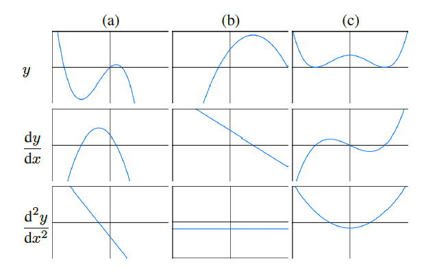
A-Diagrammatic-Construction-of-Indefinite-Integrals-Figure-4 — *Figure 4: The derivative puzzle solved so that below each graph its first and second derivative is found.*

Students tend to tackle this activity well, aided by their knowledge of quadratics and cubics, though some need time to realise that they need to determine the orientation of the given cards. The most common mistake is to place the graph of the horizontal line corresponding to the gradient function of a straight line with negative gradient the wrong way around, i.e. a horizontal line for a positive $y$ as shown in graph (2) of Figure 3. The solution of the derivative puzzle is shown in Figure 4 and the correct orientation of the horizontal line is seen in column (b).

The elusive $+C$

The final activity should be a straightforward follow-on from the derivative puzzle but it is in fact surprisingly challenging. Students are now presented with three quadratics (Figure 5, blue lines) that differ in the number of real roots, i.e. quadratic (a) has two distinct real roots, quadratic (b) has one repeated root, and quadratic (c) has no real roots. They are asked to sketch the cubic whose gradient function corresponds to each given quadratic. No equations are given and the coordinate axes are again blank to discourage an algebraic approach. The quadratics are:

Quadratic 5(a) with two distinct real roots proves to be fairly straightforward since it is similar to the curves in the derivative puzzle. After the stationary points of the cubic are determined and its intervals of increase and decrease are identified, students are generally able to sketch a cubic with two stationary points that are aligned with the roots of the quadratic.

Quadratic 5(b) with one repeated root begins to generate a little more discussion. This type of quadratic is not featured in the derivative puzzle. Furthermore the corresponding cubic is an increasing function so the stationary point is neither a maximum nor a minimum point of the curve. Here it becomes clear that students think of cubics as a curve with two stationary points and therefore some struggle to identify this cubic as a transformation of $y = x^3$ . It is however a function they are familiar with so the solution is likely to emerge from collaborative work.

Quadratic 5(c) with no real roots causes havoc even though it follows naturally from the previous case. The concept of a cubic with no stationary points seems to be new to most of my students – I can only infer that it has sadly vanished from the mathematics classroom. With some guidance, students realise that the cubic function is strictly increasing so it could be similar to the previous case. However the gradient is never zero so at the point of inflection the cubic is not ‘flat’. Eventually, and with some help, students are able to sketch the cubic. The taboo cubic is thus born. I coined this term to refer to cubics with no stationary points because we seem to never talk about them!

The main point of this activity is to present the students with a diagrammatic representation of indefinite integrals. However at no point is integration mentioned. When students are working on quadratic (a), discussion about where the corresponding cubic should be placed in the diagram often arises. Does it cross the origin? Can we determine its roots? It is a common assumption that the curve should cross the origin. Quadratic (b) generates less discussion regarding translations in the $y$ direction with most students placing the stationary point of the cubic at the root of the quadratic. In quadratic (c), the taboo cubic is in itself the main challenge but, once students arrive at it, the placing of the taboo cubic presents few issues. Figure 5 (red lines) shows examples of students’ work.

At this point, some students realise that one of the key aspects of the problem is to align the stationary points of the cubics with the roots of their corresponding quadratic and, in the case of the taboo cubic, to align its point of inflection with the vertex of the quadratic. Furthermore translations in the $y$ direction of the cubic graphs do not affect their gradient function. Time is ripe for a whole group discussion.

Collectively the group should now be able to piece together the jigsaw. My strategy is to present the group with their inevitably varied solutions and discuss which are correct and which are not. The first cubic with two stationary points usually gives away the game. Which solutions are correct? Can the cubic cross the origin? Thinking about calculus, what are we doing when we draw the cubic? ‘We are integrating, sir.’ If we are integrating, why does a translation in the $y$ direction not matter? With anticipation, I eagerly wait for the $+C$ which, to my satisfaction, has never failed to materialise so far. And so we have pinned down the elusive $+C$ . Figure 5 shows some typical students’ solutions reproduced using graphsketch.com.

Another outcome of this activity is the classification of cubics by the number of stationary points. Students are well versed in classifying quadratics by the number of real roots and its correspondence with the value of the discriminant. Classifying cubics is a natural extension of this and a very important one too as it deepens the connection between these two mathematical objects.

A-Diagrammatic-Construction-of-Indefinite-Integrals-Figure-5a — *(a)*

A-Diagrammatic-Construction-of-Indefinite-Integrals-Figure-5b — *(b)*

A-Diagrammatic-Construction-of-Indefinite-Integrals-Figure-5c — (c)
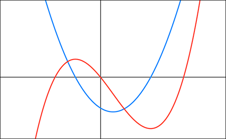
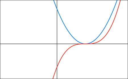
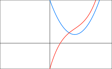
Figure 5: Three gradient functions (blue lines), with the task to find the corresponding cubic. Typical students’ solutions are shown in red.

4. What to do next and a conclusion of sorts

I follow this lesson with an activity that makes the connection between the diagrammatical and the algebraic approaches. Using examples from the MIT video lecture on Curve Sketching [6] available on the MIT Open Courseware website, I pose the following question:

By investigating their first derivative, sketch the graphs of the following functions indicating any stationary points and points of inflection:

(a) $y = {3x - x^3}$ .

(b) $y = {x^3 - 3x^2 + 3x}$ .

(d) $y = {x^4 - 4x^3 + 10}$ .

These are examples of cubics with two stationary points, one stationary point and no stationary points, and a quartic for good measure, in this order. Once presented with algebraic objects, the tendency is for students to disconnect from the diagrammatic equivalents even in a question that requires graph sketching. I find that students who combine the diagrammatic approach with the algebraic approach, i.e. students who sketch the gradient function followed by the cubic graph, are more likely to identify the point of inflection of the cubics successfully than those who rely on algebra only.

This article suggests a series of activities that lead to the diagrammatic representation of indefinite integrals and shed light on the elusive constant of integration. By exploring the geometrical nature of the gradient function, and the invertibility of differentiation and integration, we discover these concepts in a purely pictorial approach devoid of any algebra.

One of the thrills of mathematics is to make connections between topics, concepts and representations. Not only does using multiple representations enhance understanding but it also makes mathematics more exciting. And our ultimate aim should be getting our students excited about maths.

Luciano Rila
UCL and Further Maths Support Programme

References

Narrath, W. and Simonovits, R. ( $2007$ ) Instantaneous rate of change: exploring more functions with the first and second derivatives, Wolfram Demonstrations Project, http://tinyurl.com/Wolfram-derivatives.
Tall, D. (2009) Dynamic mathematics and the blending of knowledge structures in the calculus, ZDM – Int. J. Math. Educ., vol. 41, no. 4, pp. 481–492.
Mason, J. (1998) Doing and Undoing, Centre for Mathematics Education, Open University.
Swan, M. (2005) Improving Learning in Mathematics: Challenges and Strategies, Teaching and Learning Division, Department for Education and Skills Standards Unit, Sheffield.
Differentiation 1, www.univie.ac.at/moe/galerie/diff1/diff1.html, Maths Online.
Jerison, D. (2006) Lecture 10: curve sketching, MIT Open Courseware, http://tinyurl.com/MIT-curvesketching.