Incomplete Pairwise Comparison

Premier League

The English Premier League in football was interrupted by the coronavirus on 10 March. By the time this article is published it might well have restarted, but a valid question is how to extrapolate to an end result from what was already played.

Each team is supposed to play each other team twice: once at home and once away. Officially, the outcome of the season is decided on the basis of the sum of points, with 3 for a win, 1 for draw and 0 for a loss. If there is a tie it is decided on goal difference. If there is still a tie it is decided by goals for. If there is still a tie and it matters for championship or relegation then there are some subsidiary rules ending with a possible play-off.

I shall take a different criterion, namely to infer team strengths from goal differences. If each team played each other team twice as intended, then one could just add up the goal differences for a team’s matches (given team’s score minus opponent’s score) and that would give a measure of its strength. But with the season incomplete, this would not be a fair reflection: some played different numbers of matches from others, some had potentially easier fixtures left, others harder ones.

Instead, we can infer strengths $S_m$ for each team $m$ by postulating a model of the form

(1) $\begin{equation*} G_{mn} = S_m-S_n + \varepsilon_{mn} \end{equation*}$

for the goal difference of a match where $m$ plays $n$ . Here $S_m$ is a notional strength for $m$ and $\varepsilon_{mn}$ reflects a random deviation from the difference in strengths (and also rounding to produce an integer). To distinguish between the two matches where $m$ plays home or away, we will write the home team first. Let us introduce a matrix $W_{mn}$ to indicate which matches were played, with $W_{mn} = 1$ if $m$ played at home against $n$ , $0$ otherwise. Then we can determine the strengths by minimising the sum of squares

$\sum_{mn} W_{mn}(G_{mn}-S_m + S_n)^2$

over $\boldsymbol{S}$ (without loss of generality we put $G_{mn} = 0$ if the match was not played).

Least squares minimisation leads to the linear system:

(2) $\begin{equation*} \Lambda \boldsymbol{S} = \boldsymbol{U}, \end{equation*}$

with the graph Laplacian

$\Lambda_{mn} = D_{mn}-W_{mn}-W_{nm},$

where $D$ is diagonal with elements $D_{mm} = 2\sum_n W_{mn}$ , and the imbalance vector

$U_m = \sum_n G_{mn}-G_{nm}.$

There is an obvious degeneracy for (2): if $\boldsymbol{S}$ is one solution and $c$ is a constant then $\boldsymbol{S} + c \textbf{1}$ is also a solution, where $\textbf{1}$ is the vector of all 1s. But we could apply a shift to enforce the average of $S_m$ to be zero. Let $\mathcal{G}$ be the undirected graph with an edge from $m$ to $n$ if and only if they played a match. A nice theorem is that if $\mathcal{G}$ is connected then there is a solution $\boldsymbol{S}$ of (2) and it is unique up to a shift. To compute it, one can replace any of the rows of the system (2) by $\sum_m S_m = 0$ . Alternatively, to keep symmetry, one can augment $\Lambda$ by a row of 1s and a column of 1s apart from a new diagonal element of 0. Let’s say we put them in row and column 0, and augment $\boldsymbol{U}$ by a new element of 0, and solve

$\left[\begin{matrix} 0 & \textbf{1}^T \\ \textbf{1} & \Lambda \end{matrix}\right] \left[\begin{matrix} S_0 \\ \boldsymbol{S} \end{matrix}\right] = \left[\begin{matrix} 0 \\ \boldsymbol{U} \end{matrix}\right]$

for the vector $\boldsymbol{S}$ augmented by $S_0$ . Its new element $S_0$ comes out to be 0 because $\sum_m U_m = 0$ .

Note that if all matches had been played then $\boldsymbol{S} = \boldsymbol{U}/(4N-2)$ is a solution, where $N$ is the number of teams. This corresponds to dividing the total goal difference for each team by the number of matches played. But the advantage of the method is that we can apply it to an incomplete season, as long as enough matches have been played to make the graph $\mathcal{G}$ connected.

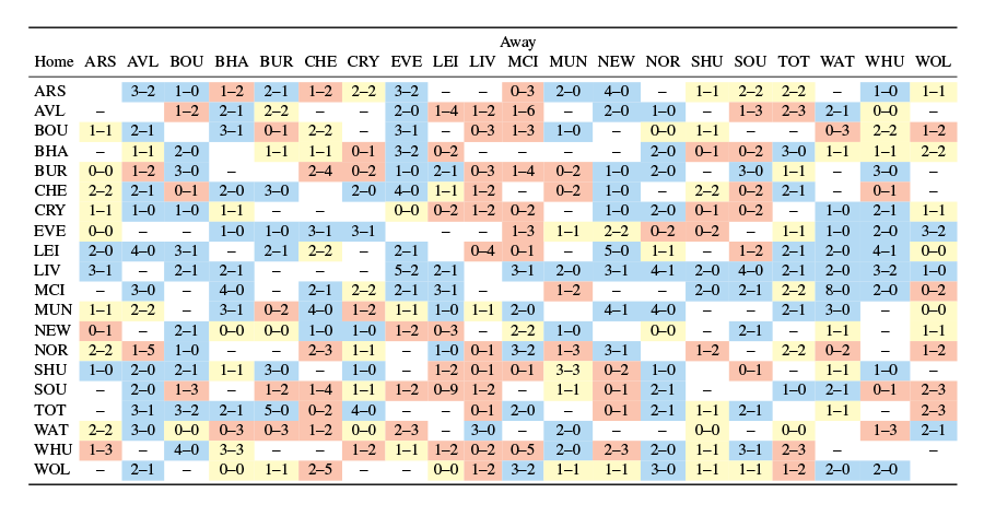
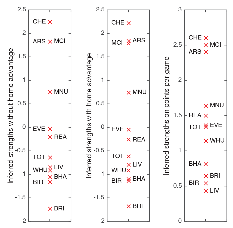
Let us apply this to the Premier League as it stood on 9 March. The scores are shown in Table 1. The results of our method are shown in the first column of Figure 1.

Premier League results before shutdown — Table 1: Premier League results 2019/20 before shutdown from Wikipedia.

Every football fan knows, however, that there is a home advantage, meaning that we should modify the model from (1) to

$G_{mn} = S_m-S_n + b + \varepsilon_{mn}$

with the home advantage $b$ to be determined as well as the strength vector $\boldsymbol{S}$ . Minimising the sum of squares again yields a slight modification of (2), which determines $b$ and $\boldsymbol{S}$ up to a shift. The modified system is

(3) $\begin{equation*} \left[\begin{matrix} \Lambda & \boldsymbol{h} \\ \boldsymbol{h}^T & w \end{matrix}\right] \left[\begin{matrix} \boldsymbol{S} \\ b \end{matrix}\right] = \left[ \begin{matrix} \boldsymbol{U} \\ g \end{matrix}\right], \end{equation*}$

where $\boldsymbol{h}$ is the vector showing the number of home matches played by each team minus the number of away matches, $w$ is the total number of matches played, and $g$ is the total goal difference (home minus away goals). Again, one can take care of the shift by enforcing $\sum_m S_m = 0$ in either of the two ways above.

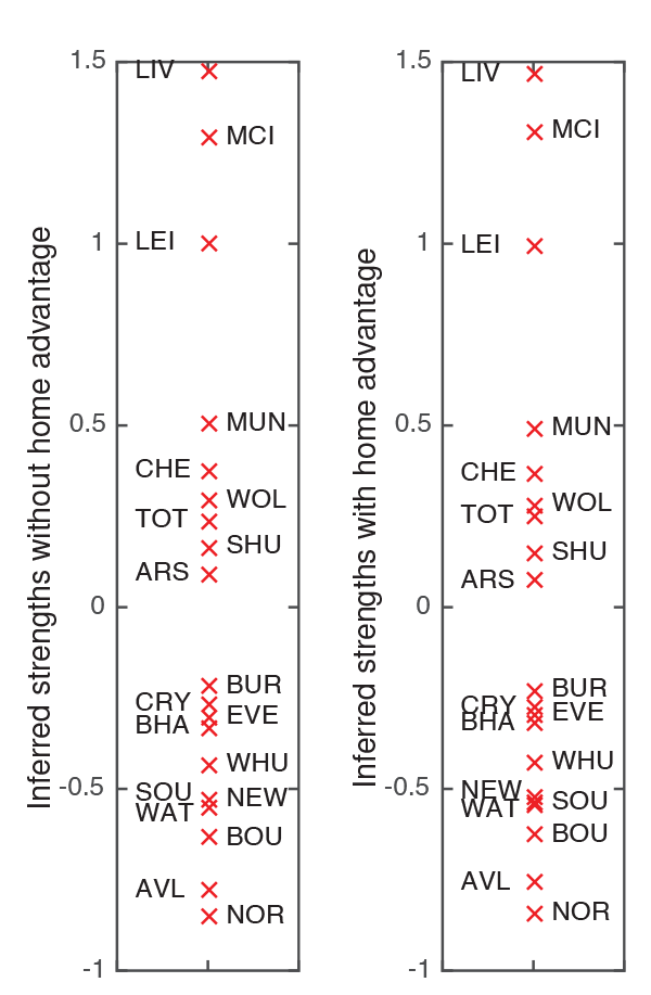
Premier League inferred stengths — Figure 1: Inferred stengths, without and with an inferred home advantage of 0.274, for the results in Table 1.

Carrying out the inference of both strengths and home advantage for this year’s Premier League produced the last column in Figure 1. The inferred home advantage was 0.274, but it can be seen that it makes hardly any difference to the inferred strengths. Presumably this is because each team had played roughly the same numbers of home and away matches.

Women’s Super League

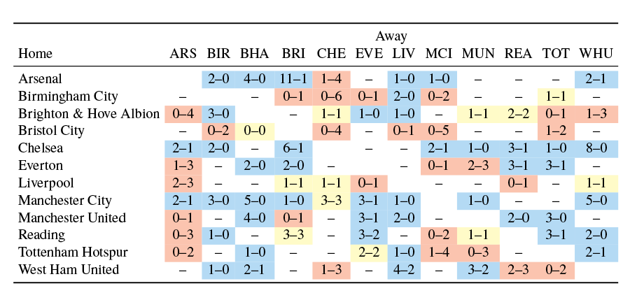
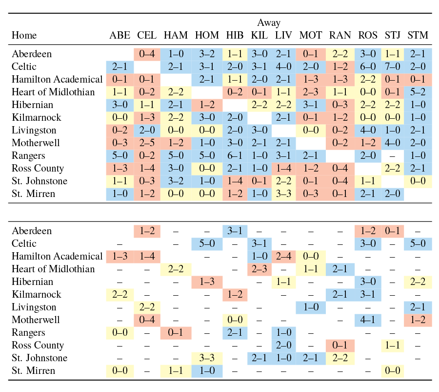
We can do the same for the Football Association Women’s Super League. It was decided on 25 May not to restart the season. So here is what my method proposes. Table 2 shows the scores when the season was suspended. Figure 2 shows the inferred strengths of the teams without including a home advantage and the strengths with an inferred home advantage, which this time comes out to be 0.380.

On 5 June the outcome was decided on points per game. This is shown in the third column of Figure 2. It shows a significant difference between inferring strengths from goal differences versus points per game. In particular, Liverpool went down to the bottom, despite not too bad goal difference. The photo is evidence for their scoring.

FA Women's Super League inferred stengths — Figure 2: Inferred strengths, without and with an inferred home advantage of 0.380, and on points per game, for the results in Table 2.

What justification does the method have? If we imagine that the goal difference could be any real number, rather than an integer, and that the deviations from strength difference are independent Gaussians with mean zero and common variance, then least squares fitting corresponds precisely to Bayesian inference of the strengths with flat prior. This result extends to the case with home advantage if we take a flat prior for it too. One could take a Gaussian prior for the home advantage and deduce a slightly modified linear system for the strengths and home advantage, but it did not seem particularly worthwhile to me. In reality the goal differences are integers and a more sophisticated probabilistic model for how the strengths produce goal differences (or even the individual goals for and against) is required, and then Bayesian inference would produce a different answer. But our method has the advantage of simplicity and relative ease of understanding.

Scottish Premiership

What about the Scottish Premiership? There, the rules are different. In phase 1, each team plays each other team three times: once home and twice away or vice versa. In phase 2, the teams are divided into a top and a bottom section and each team plays each other in the same section once, the venue being chosen to rebalance the home and away matches for the pair if possible. The Scottish Premiership was interrupted when phase 1 was not quite complete; phase 2 had not yet started. The scores are shown in Table 3.

An easy modification to the method takes care of this. We let $W_{mn}$ be the number of matches played by $m$ at home against $n$ , and $U_m$ be the sum of the goal differences over all matches played by $m$ . Then (2) gives inferred strengths for the teams. Once more, we can allow for a home advantage. It comes out to be 0.386, but again makes little difference to the inferred strengths. The results are shown in Figure 3.

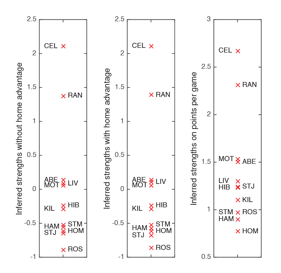
Scottish Premiership inferred stengths — Figure 3: Inferred strengths, without and with an inferred home advantage of 0.386, and on points per game, for the results in Table 3.

It was decided on 18 May to abandon the Scottish Premiership season, and settle the outcome on the basis of average points per game. The points per game are represented in the final column. One sees that there are some substantial differences: HOM is at the bottom instead of ROS, and STJ comes much higher up.

The big defect of my method, as we have seen already with the Women’s Super League, is that the real football leagues are decided on points, not goal differences. That could be addressed by formulating a probabilistic model of points as a function of strengths and doing Bayesian inference. Indeed there is a large literature on methods to infer rankings from pairwise comparisons with just win/lose outcomes. Many of the methods require a complete set of pairwise comparisons, but some do not, notably the classic [1]. A more recent reference is [2], which promotes the Borda count, being the number of matches won by a given team, as a fair measure of strength, regardless of whether there is a complete set of comparisons. To incorporate the possibility of draws in the Borda count, one could consider a draw to be equivalent to a non-match. But neither of these address the issue that a draw in the football leagues gives fewer points than the average of a win and a loss.

While finalising this article, however, I came across the blog by David Firth [3], which treats draws properly and I recommend it for further reading. He even gave a talk on it to the West Midlands branch a year ago.

Voting

The issue of inferring strengths from a set of pairwise comparisons comes up in a wide range of other contexts besides sports. For example, a market survey might produce an incomplete set of pairwise comparisons of products by a selection of consumers. A ballot might produce an incomplete set of rankings of candidates by constituents, which can be considered as providing pairwise comparisons, either by a win/loss for which candidate was ranked higher by a constituent, or by counting the difference of the ranking and using it like goal difference. Indeed, the Borda count is named after Jean-Charles de Borda who developed it in 1770 to decide on elections to the French Academy of Sciences. Historians trace its use back to the Roman Senate, and variants are used for various elections today. But I am particularly keen to use available quantitative information rather than just win/lose, which is why I promote my method.

The method is an outgrowth of one for inferring heights of nodes in a directed graph, which we call trophic analysis [4], in a project supported by the Economic and Social Research Council under grant ES/R00787X/1. If one has more information than just pairwise comparisons, say scores by panel members for incomplete selections of REF outputs and their confidences in their scores, then another step of analysis is required. In [5], we provided a method for that, which has been mentioned previously in this magazine [6].

Robert S. MacKay FRS, CMath FIMA
University of Warwick

Acknowledgements

I am grateful to Alex MacKay and Bazil Sansom for help getting the data into MatLab.

References

Bradley, R.A. and Terry, M.E. (1952) Rank analysis of incomplete block designs I. The method of paired comparisons, Biometrika, vol. 39, pp. 324–45.
Shah, N.B. and Wainwright, M.J. (2018) Simple robust and optimal ranking from pairwise comparisons, J. Mach. Learning Res., vol. 18, pp. 1–38.
Firth D. (2020) The mathematical method explained, alt-3 blog.
MacKay, R.S., Johnson, S. and Sansom, B. (2020) How directed is a directed network? arXiv preprint.
MacKay, R.S., Kenna, R., Low, R.J. and Parker, S. (2017) Calibration with confidence: a principled method for panel assessment, R. Soc. Open Sci., vol.‍ 4, 160760.
MacKay, R.S., Kenna, R., Low, R.J. et al. (2016) Calibrate with Confidence (Letter), Math. Today, vol. 52, no. 4, p. 199.