A Tennis Assignment Algorithm

For some years, I have played social tennis at a local club and have recently organised midweek men’s doubles matches for those who are retired, work part-time or have flexible working arrangements. This used to consist of asking each member of the group about their availability in the coming week, and how much they would like to play, and from their responses, putting together a set of fours using just pen and paper. However as the numbers increased, I started to think about how I could make the process easier and more efficient by writing some code and treating it as an optimisation problem. This article describes how I tackled the problem.

The initial purpose of the algorithm was to automate what I had done manually, by finding a feasible assignment of players to groups across the week and to maximise the number of groups formed. As it is clear that generally there are many possible solutions, the next step was to remove any bias or favouritism in the choice of the groups, by generating all possible feasible and equally-optimal assignments and choosing randomly from them.

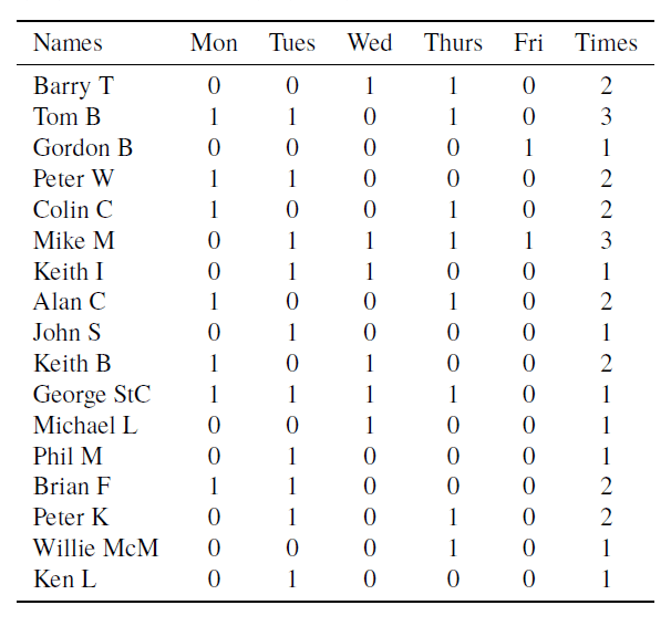
tennis-assignment-algorithm-table-1 — *Table 1: The player availability matrix $A_{ij}$*

The player availability matrix $A_{ij}$ consists of 0s and 1s, with a 1 indicating that player $i$ ( $= 1, \dots, M$ ) is available to play on day $j$ ( $= 1,\dots, N$ ). See the example in Table 1. The column on the right shows $T_i$ the maximum number of times in the week that the player has indicated that he is willing/able to play.

The variables in the problem are denoted by $x_{ij}$ which are 1 if player $i$ is assigned to play on day $j$ and zero otherwise, and are only defined for those cells where $A_{ij} = 1$ ; plus $g_j$ , the number of groups assigned to play on day $j$ . There are then two sets of constraints: firstly on the number of times in the week that a player is assigned to play (which should not exceed the maximum specified):

(1) $\begin{equation*} \Sigma_jx_{ij} \le T_i \quad \text{for} \quad i = 1, \dots, M \end{equation*}$

and secondly on the number of players assigned to play on each day which of course must be a multiple of 4:

(2) $\begin{equation*} \Sigma_{i}x_{ij}-4g_j = 0 \quad \text{for} \quad j = 1, \dots, N. \end{equation*}$

The objective is to maximise the total number of player-games in the week whilst satisfying these constraints. So we want to maximise the objective function:

(3) $\begin{equation*} z = \Sigma_{ij}x_{ij}. \end{equation*}$

This is a linear programming problem with some of the variables, the $x_{ij}$ , being binary (0-1) variables, and the rest, the $g_j$ , being integer variables. It can be solved in the software package R [1] by using the lp function (part of the lpSolve package, which is a mixed integer linear programming solver [2]) and taking as input the availability matrix in the form of a .csv file. The constraints matrix and right-hand side constants are constructed from the coefficients in (1) and (2), and the coefficients in the objective function (3) consist of 1s in front of each of the variables. For the availability matrix shown in Table 1, it turns out that $z_\text{max} = 24$ : that is, six groups can be formed over the week. One such optimal solution is shown in Table 2.

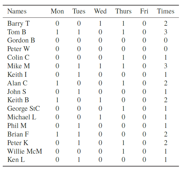
tennis-assignment-algorithm-table-2 — *Table 2: One possible optimal solution*

But there will generally be other, equally-optimal solutions (that is, different sets of $x_{ij}$ that also provide an objective function value of 24, and satisfy the constraints). To generate all or at least a sufficiently large number of the other equally-optimal solutions, the following procedure is used. Each of the coefficients in the objective function is randomly perturbed (adding or subtracting small random quantities to the base values of 1s), and the optimisation problem re-solved in a number of replications. This is done to mimic some small amount of favouritism being attached to different players and different days, whilst ensuring that the same maximum number of groups is produced.

tennis-assignment-algorithm-table-3 — Table 3: The final assignment of groups

In each replication, the solution produced is compared with all the previously-generated different solutions and is only retained if it is different from all previous ones. In this example, a total of 73 different and equally-optimal solutions were obtained. But a comparison of solutions might reveal that in one solution players A and B each play once in the week, whereas in another solution (identical in all other respects) A plays twice whilst B does not play at all. On grounds of equity this latter case is undesirable, so for each of the equally-optimal solutions we calculate $G_1$ the number of players who get at least one game. In the solution shown in Table 2, $G_1 = 15$ whilst in some other possible solutions $G_1 = 16$ . In an extension to this idea there might be a solution in which A and B each get two games in the week whilst in a different solution (again identical in all other respects) A gets three games whilst B only gets one. 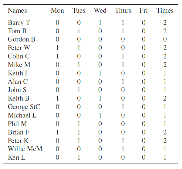So to compare the equally-optimal solutions further we calculate, for each solution, $G_2$ , the number to get at least two games. Then we sort the equally optimal solutions by descending value of $G_1$ using the value of $G_2$ to break ties. It is then found that the four best solutions have $G_1 = 16$ and $G_2 = 8$ . The final choice is made randomly from these four, and is shown in Table 3.

To complete the process, the final set of groups is printed out, ready to be copied and pasted into the email message to all members of the group:

Mon: Peter W, Colin C, Keith B, Brian F
Tues: Tom B, Peter W, Mike M, John S, Phil M, Brian F, Peter K, Ken L
Wed: Barry T, Keith I, Keith B, Michael L
Thurs: Barry T, Tom B, Colin C, Mike M, Alan C, George StC, Peter K, Willie McM

The process, which has considerably simplified my task of organising the groups each week, has worked well now for some time and whilst many members of the group are intrigued or amused to know that the assignment of players to groups is done by an algorithm, they appear to have trust in the fairness and efficiency with which it produces the results.

Mike Maher FIMA

University College London

References

R Core Team (2012) R: A language and environment for statistical computing, R Foundation for Statistical Computing, Vienna, Austria, ISBN 3-900051-07-0, www.R-project.org/.
Berkelaar, M. et al. (2013) lpSolve: Interface to Lp_solve v. 5.5 to solve linear/integer programs, R package version 5.6.7. CRAN.R-project.org/package=lpSolve.

Reproduced from Mathematics Today, October 2016

Download the article, A Tennis Assignment Algorithm (pdf)