From Mudslides to Custard: the Maths of Slurries

Suspensions of solid particles in a liquid occur just about everywhere, from mudslides to coal slurries and custard to paint. They show a very wide range of physical behaviours, some of which are surprisingly difficult to model mathematically.

Practically speaking, the applications of suspensions range from things like muddy water or whitewash – which are nearly all water with a small solid component – to pastes and cements, which have such a high solids content that they barely flow at all. These dense suspensions have lots of interesting behaviour; but the dilute suspensions are much easier to study, so let’s start there.

The ultimate limit of a dilute suspension is one where the concentration of solids is so small that it is essentially zero, and our suspension just behaves like the suspending fluid. Let’s suppose this is a Newtonian fluid (like water) with viscosity (the measure of its thickness) $\mu$ .

The first genuine question is: what happens when you add particles so sparsely that each one can be treated as if it’s the only particle in the system? Einstein [1] solved this for spherical particles in 1906 (and corrected it in 1911, which just goes to show that all scientists, even the best, make mistakes from time to time). His argument goes like this: to measure the viscosity of a fluid, we need a flow whose strain rate (the spatial derivative of the fluid velocity) is uniform in space, so that when we work out the spatial average of the stress, we have something to compare it with. This means imposing a velocity far from our particle:

$\boldsymbol{u}^\infty = \boldsymbol{U}^\infty + {\mathbf{\Omega}}^\infty\cdot \boldsymbol{x} + \boldsymbol{E}^\infty \cdot\boldsymbol{x},$

where $\boldsymbol{x}$ is the position vector of the point where we want to know the velocity, and all of $\boldsymbol{U}^\infty$ , ${\mathbf{\Omega}}^\infty$ and $\boldsymbol{E}^\infty$ are constants. Here $\boldsymbol{U}^\infty$ is a vector, ${\mathbf{\Omega}}^\infty$ is an antisymmetric matrix (representing rotation) and $\boldsymbol{E}^\infty$ is a symmetric matrix (representing a stretching flow). The most common flow used to measure viscosity in experiments is simple shear:

$\boldsymbol{u}^\infty = \dot{\gamma}y \boldsymbol{e}_x,$

for which we would have:

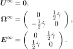
$\begin{align*} \boldsymbol{U}^\infty &= \boldsymbol{0},\\ {\mathbf{\Omega}}^\infty &= \left( \begin{array}{cc} 0 & \frac{1}{2}\dot{\gamma} \\ -\frac{1}{2}\dot{\gamma} & 0 \end{array}\right),\\ \boldsymbol{E}^\infty &= \left( \begin{array}{cc} 0 & \frac{1}{2}\dot{\gamma} \\ \frac{1}{2}\dot{\gamma} & 0 \end{array}\right). \end{align*}$

Now suppose we put a spherical particle at the origin of this flow field. If it has no external forces and torques acting on it, it will go with the flow as far as it can – it will translate with velocity $\boldsymbol{U}^\infty$ and rotate as imposed by ${\mathbf{\Omega}}^\infty$ . The only thing it can’t do is deform with $\boldsymbol{E}^\infty$ , because it’s a solid. So the extra stress (a quantity $\boldsymbol{S}$ known as the stresslet) caused by the particle ends up proportional to $\boldsymbol{E}^\infty$ :

$\boldsymbol{S} = \frac{20}{3}\pi\mu a^3 \boldsymbol{E}^\infty,$

where $a$ is the radius of the spherical particle. When we add up all these contributions over the many particles in the fluid, if the volume fraction of particles is $\phi$ then the total viscosity of the suspension becomes

$\mu \left( 1 + \frac{5}{2}\phi \right).$

The extra term is known as the Einstein viscosity, and because of its simplicity it is widely used in simulations to give a feel for the first effects of adding solids to any system.

The next level of complexity is to consider particles which are just frequent enough that each one might ‘meet’ one other particle, but no more. This one took until 1972 to be solved [2], and the calculation is much more complex. For each pair of particles positioned at, say, $\boldsymbol{x}$ and $\boldsymbol{x} + \boldsymbol{r}$ , they will each create the Einstein stress they would have done in isolation, but there’s an additional stresslet term caused by their interaction – we call it $\boldsymbol{S}(\boldsymbol{r})$ . To find the average extra stress, we need to weight this with the probability that a pair of particles will be found in that particular arrangement: we call that $P(\boldsymbol{r})$ . The trouble is, $P(\boldsymbol{r})$ is undetermined unless every particle trajectory in the system comes from infinity. That’s true for a pure stretching flow, but as soon as there’s a rotational component ${\mathbf{\Omega}}^\infty$ we’re stuck. And that, sadly, includes the very useful case of shear flow.

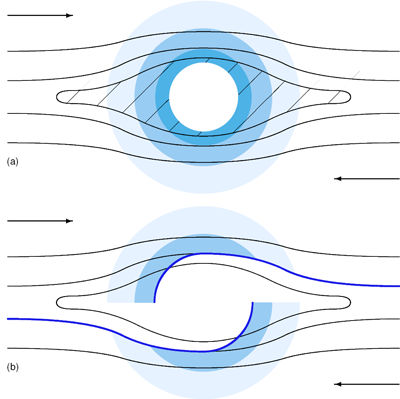
However, there is one special case where it can be rescued [3]. If we have a single layer of particles in a shear flow, the trajectories look (schematically) like Figure 1(a). The hatched region shows closed trajectories: pairs of particles which orbit around one another without ever getting very far apart. These are the places where we can’t find $P(\boldsymbol{r})$ . But if the particles repel each other very slightly if they get too close, then we get something like the picture in Figure 1(b). As the trajectories are approaching, the particles spend a long time in the close region and get held apart by the inter-particle forces; whereas when the trajectories are separating, the particles separate fairly quickly and don’t really notice the extra force. But those closed orbits can be broken by the repulsion, and suddenly we can find $P(\boldsymbol{r})$ everywhere, and calculate the viscosity to order $\phi^2$ ! We found that the larger the repulsive force, the lower the viscosity. This seems surprising but in fact it does make physical sense, because very close pairs of particles dissipate lots of energy in the thin region between the particles, and we have forced them to be further apart.

Figure 1: Pair distribution function (PDF) for the position of a sphere relative to another identical sphere in shear flow. (a) Without inter-particle forces. The barred region shows paths in which particles stay within a bounded distance forever and never escape to infinity, on which the PDF cannot be determined. (b) With a repulsive inter-particle force at close approach. Particles which would have been on closed trajectories are repelled onto an unbounded trajectory.

This is all well and good, but working with dilute systems and individual particle interactions will never get us to where the really interesting phenomena happen, which is in concentrated suspensions. The science fair example here is a cornflour-and-water mixture: stirred gently it behaves like a fairly thick liquid, but if you move too fast it solidifies and shatters like a solid. This is a jamming phenomenon known in the field as discontinuous shear thickening (or DST for short).

The physical explanation of DST has only been clarified very recently, through a combination of experimental work and theoretical insights. A key component is contact between the different particles, with friction that only acts if the particles are being squeezed together hard enough by the flow. This switching on of friction distinguishes between slow and fast flows, and produces a system that can behave quite differently in the two different cases.

One natural question to ask is, what volume fraction produces a jammed system? The answer to this turns out to depend on the type of contacts between the particles. If the inter-particle contacts each provide a pure pushing force along the line of centres, then the system will jam when the concentration is such that each particle has (on average) six contacting neighbours. But if each contact has sufficient friction that it can force the two particle surfaces to roll (rather than sliding) past one another, the number of contacts you need to jam the system goes down to just four. This means that frictional systems will jam up at a volume fraction rather lower than friction-free systems.

This argument has been developed by physicists [4] into a beautiful model that captures the behaviour of cornstarch in a steady shearing flow really well. But how do we extend it to deal with other flows?

The answer comes back to the way we were thinking about dilute systems! How do we assess how many contacts each particle should have? Through the pair distribution function $P(\boldsymbol{r})$ . We have to change things a bit: we now only care about pairs which are touching, not those that are well separated. Looking back at Figure 1(b), what we really want to know is how much probability is focused on the thick blue arc, and how it is distributed around the arc. When we were solving that problem in the dilute case, we found that (as you would expect) probability builds up in the compressive zone as the background flow wants to push particles together; and dissipates in the extensional zone as the flow naturally pulls particles apart.

We can characterise these zones using the stretch matrix $\boldsymbol{E}^\infty$ . The matrix has both positive and negative eigenvalues; the compressive zone is associated with the eigenvector(s) whose eigenvalues are negative, and the extensional zone is associated with the eigenvector(s) whose eigenvalues are positive. We can split any stretch matrix into two components, one with all eigenvalues positive or zero, the other with all eigenvalues negative or zero – and then use those two matrices as part of the equations describing the evolution of $P(\boldsymbol{r})$ [5]. For the simple shear flow above, the split $\boldsymbol{E}^\infty = \boldsymbol{E}^c + \boldsymbol{E}^e$ gives:

$\begin{align*} \boldsymbol{E}^\infty &= \left( \begin{array}{rr} 0 & \frac{1}{2}\dot{\gamma} \\[2pt] \frac{1}{2}\dot{\gamma} & 0 \end{array}\right),\\ \boldsymbol{E}^c &= \left( \begin{array}{rr} -\frac{1}{4}\dot{\gamma} & \frac{1}{4}\dot{\gamma} \\[2pt] \frac{1}{4}\dot{\gamma} & -\frac{1}{4}\dot{\gamma} \end{array}\right),\\ \boldsymbol{E}^e &= \left( \begin{array}{rr} \frac{1}{4}\dot{\gamma} & \frac{1}{4}\dot{\gamma} \\[2pt] \frac{1}{4}\dot{\gamma} & \frac{1}{4}\dot{\gamma} \end{array}\right). \end{align*}$

Our use of these compression and extension matrices adapts the beautiful steady theory [4] to general flows like, for instance, a sudden reversal of the shear direction. Our predictions for the force measured in such a system are shown in Figure 2, along with the results from numerical simulations. The agreement is pleasing (though if you read the paper [5] you will find other measures on which we do less well).

Figure 2: Viscosity (relative to solvent) plotted against shear in instantaneously reversed shear flow at different dimensionless shear rates. From top to bottom, shear rates are infinity, 0.03, 0.02, 0. Data from [5].

As so often in mathematics, understanding gained in one area – in this case, the rather academic and un-applicable study of dilute suspensions – can turn out to be relevant somewhere much more useful!

It was an honour and a privilege to be invited to give the IMA Lighthill Lecture 2022 at BAMC in Loughborough. There is a display about Sir James Lighthill and his work directly outside my office at UCL, where he was Provost for 10 years. My first BAMC, as a PhD student in Edinburgh in 1997, was one of his last (he died in 1998) and he gave the final plenary lecture. His transparencies were covered with huge amounts of material in many different colours of pen, in a style that shouldn’t have worked but did. I am delighted to have had the opportunity to follow, just a little, in his footsteps.

Helen Wilson FIMA
University College London

References

Einstein, A. (1906) A new determination of molecular dimensions, Ann. Phys. (Berl.), vol. 19, pp. 289–306, Corrections (1911) vol. 34, pp. 591–592.
Batchelor, G. and Green, J. (1972) The determination of the bulk stress in a suspension of spherical particles to order $c^2$ , J. Fluid Mech., vol. 56, pp. 401–427.
Wilson, H.J. and Davis, R.H. (2002) Shear stress of a monolayer of rough spheres, J. Fluid Mech., vol. 452, pp. 425–441.
Wyart M. and Cates, M.E. (2014) Discontinuous shear thickening without inertia in dense non-Brownian suspensions, Phys. Rev. Lett., vol. 112, p. 098302.
Gillissen, J.J.J. et al (2020) Constitutive model for shear-thickening suspensions: Predictions for steady shear with superposed transverse oscillations, J. Rheol., vol. 64, pp. 353–365.