The motivating question
Why is it always the full glasses that get knocked over? That question was posed after a mildly unfortunate incident involving a glass of lemonade. I do not always tune into every nuance of a social situation, so it took me a few moments before I realised this was intended to be a rhetorical question. Nevertheless, it started me thinking. And once I had started, I found myself on something of a roll.
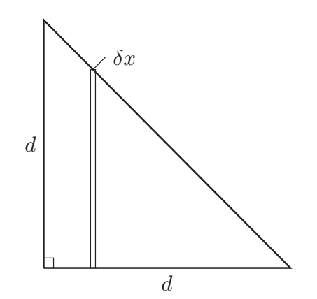
In the finest of traditions, we begin by making some simplifying assumptions. We assume that the weight of the glass is negligible compared to the weight of its contents. We also assume that the contents can be represented as a rigid column. In this situation, a glass will fall over if the centre of gravity (COG) of its contents is outside the point where the glass touches the table.

Two situations are illustrated in Figure 1. The left-hand side is vaguely representative of a full glass, the height of the column  being four times its diameter
  . The right-hand side is the same glass when it is much emptier; in this case the height and diameter are the same. It is easy to see that the tipping point occurs when
  reaches a critical value, defined by
  .
.
For the two cases shown in Figure 1, the critical angles are approximately  and
and  respectively. The much smaller angle in the first case suggests one reason why a full glass may be more likely to get knocked over than an empty one.
Of course, this explanation ignores a number of potentially important factors. Some of these were covered in our simplifying assumptions. Another relates to inertia: the fuller glass has a greater mass and hence requires a greater force to achieve a given angle between the glass and table. There may also be a psychological component: knocking over a full glass has a greater consequence than knocking over an empty one, so it may form stronger memories and hence may be judged to occur with a higher frequency than is actually the case.
Although these points are all interesting, this article will endeavour to answer a more general problem: namely, how do we calculate the COG of an arbitrary shape?
Integrating moments
Consider the triangle shown in Figure 2. This is a right-angled triangle in which the two sides neighbouring the right-angle both have length . For convenience, we assume the origin is located at the right-angled vertex and that the two neighbouring sides define the  – and
– and  -axes.
In simple terms, to calculate the co-ordinate of the COG, we sum all the turning moments (i.e. mass times distance) and divide this value, denoted  , by the mass of the triangle. Without loss of generality, we assume the triangle has unit density. Hence, rather than mass we consider area and it is trivial to see that the triangle’s area is simply
  . To sum the turning moments we consider a thin strip, of height and width
  at a distance from the origin, and also note that the triangle’s hypotenuse (and hence the height of the strip) is defined by
  . We then have:
![\begin{align*} \operatorname{SumTM} &= \int^d_0 x y \; \mathrm{d} x \ = \int^d_0 x d - x^2 \; \mathrm{d} x \\ &= \left[ \frac{1}{2} x^2 d - \frac{1}{3} x^3 \right]^d_0 = \frac{d^3}{6}. \end{align*}](https://ima.org.uk/wp/wp-content/ql-cache/quicklatex.com-dbadd8f943b677fff5442666cfcc7ff0_l3.svg "Rendered by QuickLaTeX.com")
Dividing the above result by the triangle’s area, we see that  . By symmetry, we can deduce that
  has the same value as
  , although if we really wanted to we could perform another integration to get this result.
Composite shapes
There is no reason why we cannot use integration to determine the COG of any shape. However, it is often easier to calculate the location of the COG of a composite shape via the weighted sum of its components.

Consider, for example, the planar shape illustrated in Figure 3.This is, essentially, a rectangle  with two added right-angled triangles,
  and
and  : the length
  is half that of
  ; likewise,
  is half
  . Using
  to denote mass, and subscripts to identify particular components, we can calculate the COG of the overall shape via:

We can adopt a similar approach by considering pieces that have been removed as having negative mass. As such, an equivalent way of calculating the COG would be via:

In this specific case, if we take  and as both being of unit length (along the and axes respectively) then the COG is located at approximately
  .
.
Now, assume that we set the shape rolling and, as a consequence, it is equally likely to reach an instantaneous zero velocity at any orientation; that is the angle between and the table is uniformly distributed amongst  . Obviously, most of these orientations will be unstable and the shape will eventually come to rest with a particular side on the bottom.

Given our previous discussions, it is plausible that the likelihood of the shape coming to rest with, say, on the bottom is proportional to the angle subtends from the COG. Since we know the location of the COG this angle can easily be calculated using the cosine rule. Using these assumptions provides the results shown in Table 1.
It is apparent from Table 1 that sides and have equal chance of ending up on the bottom; given the shape’s symmetry this is what would be expected. The table also shows that the chance of being on the bottom is over 7% greater than the chance of  being on the bottom.
Building blocks
Before we get on to the final piece of the article it is helpful to establish COG locations for a couple of shapes we will use as building blocks; specifically a hemisphere and a square-based pyramid.
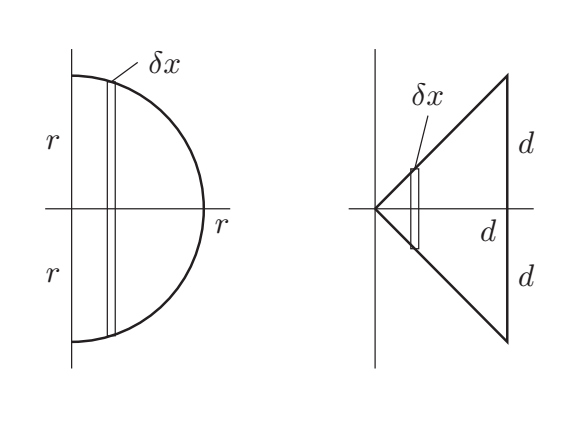
To begin with, we consider a hemisphere of radius  , as shown in the projection that forms the left-hand side of Figure 4. We take the origin as the centre of hemisphere’s base. By symmetry, we know the COG lies along the radial line that is perpendicular to this base. To determine how far the COG is from the base, we integrate across a number of discs of radius
  and width , at distance . As with the planar shape, we assume a uniform density, so mass and volume are the same.
![\begin{align*} \operatorname{SumTM} &= \int^r_0 x \pi y^2 \; \mathrm{d} x \ = \int^r_0 \pi x r^2 + \pi x^3 \; \mathrm{d} x \\ &= \left[ \frac{1}{2} \pi x^2 r^2 - \frac{1}{4} \pi x^4 \right]^r_0 = \frac{\pi r^4}{4}.\end{align*}](https://ima.org.uk/wp/wp-content/ql-cache/quicklatex.com-35f1901f3a72619a69360aaf331f2486_l3.svg "Rendered by QuickLaTeX.com")
The mass of the hemisphere is  . So, we deduce that the COG is
  away from the base.
We are also interested in a square-based pyramid of height with the sides of the square base being  in length; this is illustrated in the projection shown in the right-hand part of Figure 4. In this case we are interested in the distance between the pyramid’s apex and the COG; by symmetry we know the COG must be on the line joining the centre of the base to the apex.
Whereas for the hemisphere we were integrating discs, in this case we are integrating slim squares, which have sides of length  and width .
![\begin{align*} \operatorname{SumTM} &= \int^d_0 x 4 y^2 \; \mathrm{d} x \ = \int^d_0 4 x^3 \; \mathrm{d} x \\ &= \left[ x^4 \right]^d_0 = d^4.\end{align*}](https://ima.org.uk/wp/wp-content/ql-cache/quicklatex.com-55a34a582e0dd4d2d5d08e83fda71beb_l3.svg "Rendered by QuickLaTeX.com")
The mass of the square-based pyramid can be determined using a similar integral, which gives a result of  . Hence, the COG is
  away from the apex.
Bringing it together
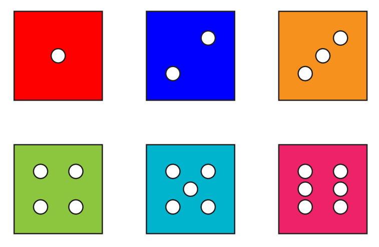
We now take six square-based pyramids, each of height  and square base 1. On the base of each pyramid we drill a number of hemispherical holes, in the arrangements shown in Figure 5; these hemispheres have radius 0.08.
Using the results discussed previously we can determine the location of the COG of each of the square-based pyramids. Note that, due to the symmetry of the drilled hemispheres the COG of each of these shapes is on the line joining the apex to the centre of the base.
We arrange the six pyramids with their apexes at a common point, which we take as the origin. The lines joining the apexes to the centre of their bases are aligned with axes as is as shown in Table 2.

This arrangement allows us to find the COG of something that is similar to a six-sided die. Completing the calculation we find the COG is actually located at  ; that is, it is not at the centre of the die.
In the same way that we used the angle subtended by a side to consider the likely final position of the planar shape, we use the solid angle subtended by a face from the COG to determine the likely final position of the die. More particularly, we split a face into two triangles and determine the angle each triangle subtends. The angle subtended by the face is simply the sum of these angles.
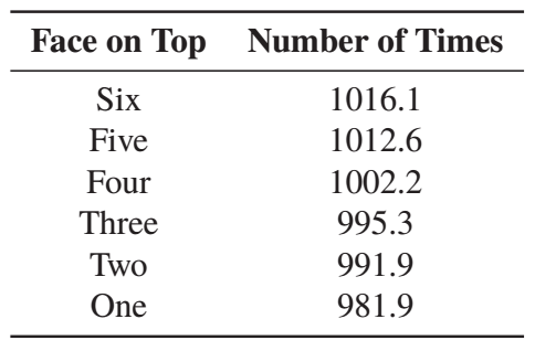
Wikipedia provides two ways of calculating these angles (https://en.wikipedia.org/wiki/Solid_angle). Within this work, both mechanisms were implemented and the results checked for consistency. Comparing the subtended angles allows us to estimate the number of times a given face will end up on top. The results for a series of 6,000 rolls are shown in Table 3.
Table 3 shows that the Six face is most likely to end up on the top. This is because the COG of our die-like shape is closer to the One face, which is thus more likely to end up on the bottom. The table shows that across 6,000 rolls Six (the most likely outcome) will be thrown approximately 34 more times than One (the least likely outcome).
It is interesting to note that the offset of the COG from the centre of the shape is exacerbated by placing the One face opposite the Six face. This is because this arrangement places the pyramid with fewest hemispheres opposite the one with the most hemispheres. I do not know why this arrangement was chosen, but it seems the standard approach.
A fairer distribution of outcomes would be achieved if the One face was opposite the Two face, the three Face opposite the Four face and the Five face opposite the Six face. In this case, across 6,000 rolls the most likely outcome occurs less than seven times more than the least likely outcome.
Future work
There are obviously lots of limitations with the discussion above. For example, die corners tend to be rounded; perhaps this rounding realigns the COG so that it is at the centre of the die. Likewise, at least in some cases, the holes on the faces are painted; perhaps the weight of the paint provides the necessary correction. Alternatively, perhaps die manufacturers place a weight at the centre of the die. Or maybe some other mechanism is used.
What is clear is that further research would be beneficial. This could even involve a field trip to Las Vegas but, if it does, please do not invite me; I would undoubtedly knock over my glass of lemonade and make a mess of the gambling table!
Rob Ashmore CMath CSci FIMA
Dstl
Notes
Strictly speaking, this article is based on the centre of mass (COM) rather than the COG. However, in a uniform gravitational field the COM and COG are coincident. Given all the other simplifying assumptions that are made, assuming a uniform gravitational field does not seem unreasonable. For that reason the more commonly understood term, COG, was adopted.
Acknowledgement
‘Urban Maths’ cartoonist: Adrian Metcalfe – www.thisisfruittree.com
The views and opinions expressed herein are those of the author and do not necessarily reflect those of Dstl.
Crown Copyright © 2017 Dstl, This information is licensed under the Open Government Licence v3.


