Designing Interplanetary Transfers

Leaving Earth and arriving at another planet or asteroid requires a spacecraft to implement a sequence of manoeuvres. These include changes of velocity needed to escape Earth, to insert into an orbit around the target and make any intermediate manoeuvres to assist in the transfer. In fact, space mission designs are often measured by a delta V ( $\Delta V$ ) or total propulsive speed change requirement of the spacecraft.

These manoeuvres are performed by a propulsion system on board the spacecraft, working on the principle of expulsion of a propellant at high velocity to provide a reaction thrust. The velocity of the propellant is determined by the type of propulsion system available on the spacecraft. Standard chemical rocket engines using the combustion of a fuel and oxidant achieve propellant speeds of typically 3,000 to 4,500 m/s. This is a measure of the specific impulse of the propulsion system, or impulse per unit mass of propellant.

The amount of propellant used to achieve a given $\Delta V$ is given by the classical rocket equation, i.e.:

$\begin{equation*}m_\mathrm{fuel} = m_\mathrm{initial}\left( 1 - \mathrm{e}^{-\frac{\Delta V}{\mathrm{Isp}}}\right),\end{equation*}$

where $m_\mathrm{fuel}$ is the propellant mass, $m_\mathrm{initial}$ is the initial mass of the spacecraft, $\Delta V$ is the delta V and Isp is the propulsion system specific impulse (measured in m/s).

The exponential relationship shows clearly that large speed changes can result in the mass available after the manoeuvre approaching zero. The key consideration is the ratio of $\Delta V$ to propulsion system specific impulse. When the mass remaining after subtraction of propellant becomes less than the mass of the spacecraft support systems and instruments, the designated transfer becomes unviable.

This means that either the required speed change must be reduced or the launch mass increased. Increasing launch mass is restricted by the capability of the launch vehicle being used and so often focus lies on constraining, or minimising, the speed change needed to execute the mission.

Therefore there is considerable interest in finding optimal transfers from launch to the mission target, that minimise the $\Delta V$ and the consequent propellant usage. To achieve this goal a number of building blocks are needed and are described in the following sections.

Simulation of interplanetary space flight

The motion of a spacecraft flying on an interplanetary mission is influenced by several forces. These are primarily gravitational and for most of the mission the Sun’s influence is dominant. Approaching the planets the local gravitational fields can dominate.

The solution of the two-body problem (spacecraft and a single gravity source) is well known and described analytically by Keplerian orbital motion. However the introduction of further gravity sources results in the need for alternative means to precisely predict the motion. The ordinary differential equation built from a Newtonian description of gravity can only be solved precisely by numerical integration methods.

The equations of motion for the spacecraft with respect to the Sun are the following:

$\begin{equation*}\frac{\mathrm{d}^2 \boldsymbol{r}}{\mathrm{d} t^2} = \frac{\boldsymbol{\mathrm{Force}}}{\mathrm{mass}} - \frac{\mu}{r^3}\boldsymbol{r} - \sum^{i = N}_{i = 1} \left[ \frac{\mu_\mathrm{pi}}{r_\mathrm{pi}^3}\boldsymbol{r_\mathrm{pi}} - \frac{\mu_\mathrm{pi}}{r_\mathrm{relpi}^3}\boldsymbol{r_\mathrm{relpi}} \right],\end{equation*}$

where $\boldsymbol{r}$ is the spacecraft acceleration with respect to the Sun, $\boldsymbol{r_\mathrm{pi}}$ is the $i$ th planet position with respect to the Sun, $\boldsymbol{r_\mathrm{relpi}}$ is the spacecraft position with respect to planet $i$ , $\mu$ is the Sun’s gravitational constant and $\mu_\mathrm{pi}$ is the $i$ th planet’s gravitational constant. Force is the vector of non-gravitational forces acting on the spacecraft.

The above terms with $\boldsymbol{r_\mathrm{pi}}$ are to account for the acceleration of the Sun caused by the corresponding planet’s gravity field.

Building blocks of interplanetary transfers

Although the precise interplanetary motion cannot be described analytically, key aspects of the transfer can be approximated and are amenable to a much simplified analysis. These simplifications are often employed in the preliminary design of interplanetary transfers.

Lambert’s problem

Designing-interplanetry-transfers-figure-1 — *Figure 1: Illustration of Lambert’s problem.*

An important problem in interplanetary mission design is to find a trajectory that leaves one planet, at a certain absolute date, or ‘epoch’, and arrives at a second planet at a later epoch. These departure and arrival epochs may be chosen freely, but have large implications for the $\Delta V$ required to implement the transfer.

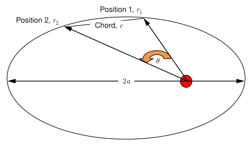
This is Lambert’s problem, which is stated as: given an initial and a final position, together with a time of flight; determine the connecting orbit. Figure 1 illustrates this. A closed orbit is assumed to link the initial position at planet 1 to the final position at planet 2, where $r_1$ is the radial distance in the spacecraft’s orbit when leaving planet 1 and $r_2$ is the radial distance in the spacecraft’s orbit when arriving at planet 2.

The solution of this problem demonstrates that the time of flight between these two positions depends upon three quantities, all defined in Figure 1.

These are:

The semi-major axis of the connecting ellipse, $a$
The chord length, $c$
The sum of the position radii from the focus or the connecting ellipse.

The length of the chord connecting the two positions is given by:

$\begin{equation*}c^2 = r_1^2 + r_2^2-2r_1r_2\cos{\theta}.\end{equation*}$

The semi-perimeter of the connecting triangle between the focus and the two points is the following:

$\begin{equation*}s = \frac{r_1 + r_2 + c}{2}.\end{equation*}$

Intermediate variables, $\alpha$ and $\beta$ are introduced.

$\begin{equation*} \sin ^2 \frac{\alpha}{2} = \frac{s}{2a} \textrm{ and } \sin ^2\frac{\beta}{2} = \frac{s-c}{2a}.\end{equation*}$

With these definitions the following expression can be obtained:

$\begin{equation*}(t_2-t_1) = \sqrt{\frac{a^3}{\mu}}((\alpha - \sin{\alpha})-(\beta-\sin{\beta})).\end{equation*}$

This equation is then solved for the semi-major axis, $a$ . An iterative procedure is needed. Convergence is made more robust via application of specialised methods.

Designing-interplanetry-transfers-figure-2 — *Figure 2: Speed change contours for an Earth to Mars transfer obtained from Lambert’s method (departure/arrival $V_\infty$ totals).*

Having found the semi-major axis further details of the transfer orbit are obtained from Keplerian orbit properties. By comparison of the velocities in the transfer orbit and in the planet orbits at the departure and arrival locations, the speed change needed by the spacecraft can be found. These heliocentric speed changes are actually a close approximation to the ‘Vinfinities’ or excess hyperbolic speeds ( $V_\infty$ ) of a hyperbolic orbit around the planet. When leaving Earth the spacecraft must reach the required hyperbolic orbit by application of a large speed increment close to its Earth orbit perigee. This can be supplied by the launcher or the spacecraft itself. Similarly, the spacecraft reaches the target planet in a hyperbolic orbit with a Vinfinity defined by the heliocentric transfer. A retro-manoeuvre is then applied on reaching the pericentre of the hyperbolic orbit. Figure 2 shows the speed change contours for a transfer from Earth to Mars obtained by solution of Lambert’s problem for a range of departure dates at Earth and transfer durations, which define the arrival date at Mars.

This remarkably powerful method allows the generation of surveys of a wide range of interplanetary transfer options spanning many launch dates. Repeated solution of Lambert’s problem over such a grid only requires seconds of computer time on a modern PC.

Two limitations exist to this method:

Only planet to planet transfers are assessed.
No manoeuvres between planets are included.

These limitations will be discussed in the following sections.

Gravity assists

In many transfers, particularly to enable reaching more distant planets, additional tools are needed. The major mission enabler in such transfers is known as the gravity assist, sometimes called a slingshot.

The interplanetary trajectory of the spacecraft can result in an orbit that crosses that of an intermediate planet. The process of a gravity assist involves the gravitational deflection of the spacecraft velocity between approaching and departing such a planet. The relative speed on approaching the planet approximates the excess hyperbolic speed $V_\infty$ of a hyperbolic orbit. The spacecraft then passes through the pericentre of the hyperbola and departs in a new direction, when viewed in a planet-centred frame of reference. The deflection angle is the difference in the asymptotic approach and departures.

On leaving the planet’s gravitational influence, the resulting velocity relative to the Sun has been modified by the change in direction relative to the planet. This effect can be approximated by the construction of two velocity vector triangles, where the total velocity relative to the Sun is the planet’s relative velocity plus the planet’s velocity. Figure 3 shows the velocity vector geometry.

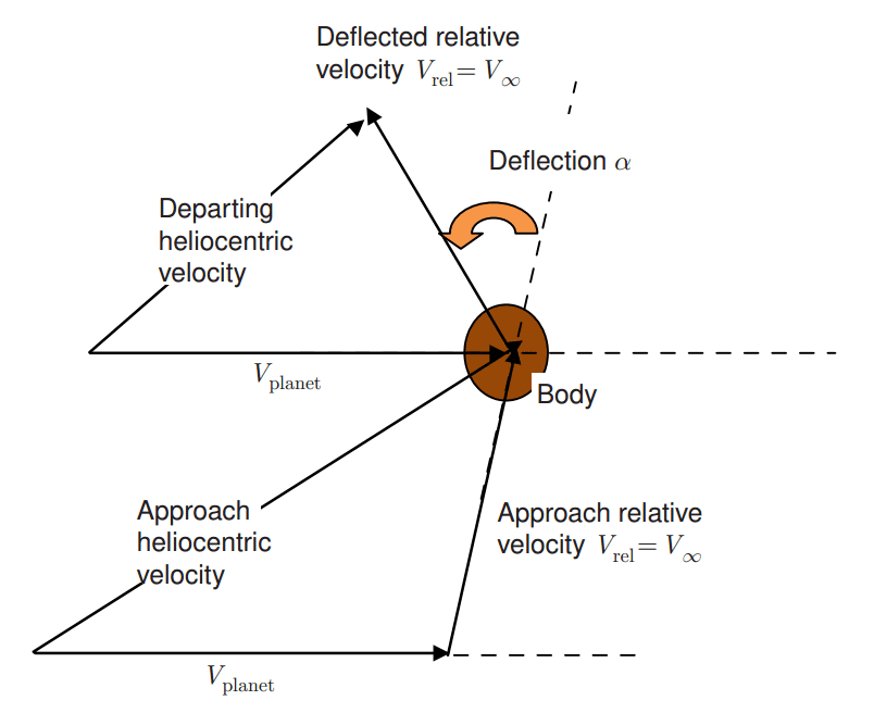
Designing-interplanetry-transfers-figure-3 — Figure 3: Example of velocity change as a spacecraft’s relative velocity is deflected by an angle $alpha$ during its hyperbolic orbit about a planet. The two velocity vector triangles illustrate the situation approaching (lower) and leaving the planet (upper). Only the asymptotic arrival and departure velocity vectors of the planet relative orbit are illustrated. In this example velocity and hence energy is reduced.

This change in velocity relative to the Sun means that the spacecraft’s Sun-relative orbital energy is modified. It can either be increased or decreased, depending on which side of the planet pericentre is targeted. Had such an orbit change been implemented by propulsion the $\Delta V$ required could be thousands of metres per second. More massive planets provide greater deflection and therefore the possibility of more ‘free’ $\Delta V$ .

This change in orbit can be used to advantageously modify the transfer. No propulsive manoeuvre from the spacecraft is needed to achieve such an effect. This is the principle of the gravity assist. Good examples are the NASA Voyager 1 and 2 missions, using multiple gravity assists in the outer Solar system to boost their energy and escape from the Solar system. ESA’s Rosetta spacecraft was able to perform a rendezvous with a comet, after performing a gravity assist at Mars and three at Earth during its transfer.

Transfer optimisation

An interplanetary mission is built up of the previously described elements: planet to planet arcs, deep space manoeuvres and gravity assist. Minimum $\Delta V$ solutions are sought to limit propellant usage and so ensure feasible spacecraft total mass.

A multi-step procedure can be used whereby once a target has been selected, a mission can be automatically designed such that the spacecraft-applied speed change, i.e. $\Delta V$ , or propellant need is minimised.

The steps are:

Identification of possible routes
Preliminary optimisation
Refined optimisation

When a target is specified, a series of possible routes can be considered. A route is principally defined as the sequence of planets used for gravity assist. A minimum $\Delta V$ solution will exist for each route.

Both global and local optima in the transfer are of interest. A local optimum can be identified for each route and the global optimum utilises the most efficient route. In many cases similar $\Delta V$ s may be found for a range of different routes. In addition to propellant usage, route variations can have a significant effect on the environment of the spacecraft during the transfer, for example, minimum and maximum distances from the Sun, maximum distance from Earth. Preliminary optimisation can be achieved by search methods utilising evaluation of transfer ‘grids’ via application of Lambert’s problem and approximation of gravity assists, or by application of global optimisation methods utilising similar approximations in the transfer. Genetic algorithms are often successfully used in the global optimisation phase because the number of optimisable variables is relatively small in the preliminary formulation.

Local optimisation

Having obtained preliminary solutions the transfer can now be modelled in greater detail using numerical integration methods. Local optimisation is now used to obtain the details needed for the spacecraft manoeuvres and ultimately the propellant needs.

The mathematical problem for local optimisation can be expressed as: minimise an objective function $J$ , typically propellant usage, with respect to a set of control parameters, $\boldsymbol{u}$ . The transfer is subject to both equality and inequality constraints.

Examples of equality constraints are departure/arrival constraints. Path constraints could, for example, be restrictions on thrust vector pointing.

An objective that often occurs in the context of interplanetary missions is the minimisation of propellant mass via maximisation of spacecraft mass at the end of the transfer. This can be obtained by numerical integration of the propellant mass flow as:

$\begin{equation*}J = \int^{t_f}_{t_0}\dot{m}(\boldsymbol{X}, \boldsymbol{u}, t) \,\mathrm{d} t.\end{equation*}$

The propellant mass flow will generally depend upon thrust and specific impulse. Thrust may have a positional dependence and is controlled in magnitude by the throttle that is applied.

$\boldsymbol{X}$ is the state vector (i.e. position, velocity, mass), $\boldsymbol{u}$ is the optimisable control vector, which will be manoeuvre details and event times, $t_f$ is the time at which the trajectory terminates and $t_0$ is the time at which the trajectory starts.

The state vector is obtained by integrating the state vector rates, i.e.:

$\begin{equation*}\boldsymbol{X} = \boldsymbol{X(t_0)} + \int^{t_f}_{t_0}\dot{\boldsymbol{X}}(\boldsymbol{X}, \boldsymbol{u}, t)\,\mathrm{d} t.\end{equation*}$

A range of methods are available to solve this optimisation problem. The control parameters can include terms that are continuously variable in time such as thrust steering angles. In this context the application of Pontryagin’s maximum principle allows solution via derivation of a set of adjoint differential equations. A two-point boundary value problem is obtained whose solution will yield the time dependence of the control elements. This method whilst mathematically elegant can be subject to numerical difficulties in convergence for many real world problems.

Therefore alternatives can be employed that involve parameterisation of the continuously variable control elements. A finite set of optimisable parameters then define the time dependence. These are so-called ‘direct’ optimisation methods and numerous versions are possible, distinguished by the methods of parameterisation and also the representation of the trajectory. For example the trajectory can be split into a number of segments that need to be linked by equality constraints in an expanded optimisation problem. The number of control parameters and constraints is increased but rates of convergence are often substantially improved.

Solutions are obtained by a non-linear programming (NLP) algorithm; an iterative procedure utilising the gradients of states, constraints and objective with respect to the control parameters.

Gradient evaluation

The Jacobian, i.e. the matrix of constraint gradients, is obtained from an extended state transition matrix, which is the matrix of partial derivatives of states at a defined time with respect to initial state values and control parameters. This matrix can be obtained either by numerical differencing or by variational methods, the latter offering the possibility of improved computational efficiency. Variational methods allow the matrix elements, i.e.\ the partial derivatives of state with respect to parameter, to be obtained by numerical integration:

$\begin{equation*}\frac{\partial X_i(t)}{\partial u_j} = \int ^t_{t_0}\frac{\partial \dot{X}_i}{\partial u_j}(\boldsymbol{X},\boldsymbol{u,t})\,\mathrm{d} t + \frac{\partial t_f}{\partial u_i}\dot{X}_i(t_f)-\frac{\partial t_0}{\partial u_i}\dot{X}_i(t_0),\end{equation*}$

where ${\partial X_i}/{\partial u_j}$ is the partial derivative of the instantaneous value of the $i$ th state element with respect to the $j$ th control parameter and ${\partial \dot{X}_i}/{\partial u_j}$ is the partial derivative of the time derivative of the instantaneous value of the $i$ th state element with respect to the $j$ th control parameter. Variational methods require greater analytical derivation than differencing methods. Alternatively automatic differentiation functions can be utilised.

The total number of optimisable parameters depends on the problem under consideration and the type of propulsion system. Low-thrust systems requiring long-term application over the trajectory require greater numbers of parameters for their representation. Numbers can range from hundreds to millions.

Non-linear programming

When the gradients of all states, constraints and the objective function are available, an increment in the control parameters can be calculated, by using an NLP algorithm, to approach the optimum solution.

The form of algorithm that is most applicable is dependent on the information available. In complex trajectory optimisation problems, it is likely that only first-order gradient information is available about the objective and constraints. This is due to the computational overhead in obtaining higher order derivatives, but depends on the detail of the optimisation method employed. However, good performance is available using only first-order gradient information.

Many NLP methods have been developed and this is a specialised subject with application to many fields of optimisation. An illustration of a relatively simple, but robust method is outlined in the following paragraphs, to illustrate some of the principles and considerations in using such algorithms. This algorithm has in fact been applied to the design of many space missions with a wide variety of applications. It has been used both in the early mission design phase and also in detailed manoeuvre design and planning.

The gradient projection method developed by Rosen uses a constrained steepest descent approach.It can be applied to a wide range of problems. The problem is to find the optimisable control parameters, $\boldsymbol{u}$ , required to meet the final state constraint vector condition: $\boldsymbol{C} = 0$ and maximise or minimise the objective, $J$ .

Given an initial estimate for $\boldsymbol{u}$ , the constraint vector $\boldsymbol{C}$ will not equal zero, but be equal to an error, $\boldsymbol{E}$ . An augmented objective can be defined by adjoining the constraint vector to the objective:

$\begin{equation*}J^* = J + \boldsymbol{\lambda ^T} \bullet \boldsymbol{C},\end{equation*}$

where $\boldsymbol \lambda$ is a vector of undetermined Lagrange multipliers.

$J^*$ can be improved by making a step $\boldsymbol{\Delta U}$ be in the direction of the gradient vector, i.e.

$\begin{equation*}\boldsymbol{\Delta U} = k \left( \boldsymbol g + {\left [\boldsymbol{\lambda ^T}A^T\right ]}^T \right),\end{equation*}$

where $k$ is a constant and $\boldsymbol g$ is the gradient vector of $J$ with respect to the control parameters. Similarly $A$ is the gradient matrix of the constraint vector $\boldsymbol{C}$ .

If an error exists in the constraint vector, i.e. $\boldsymbol C =\boldsymbol E$ , then we can also require that the step in $\boldsymbol u$ is such that it changes the constraint vector accordingly: $\Delta \boldsymbol C = - \boldsymbol E$ .

The Lagrange multipliers are then found from the following expression:

$\begin{equation*}\boldsymbol \lambda = {\left[A^TA\right]}^{-1} \left(-\frac{\boldsymbol E}{k}-A^T\boldsymbol g \right).\end{equation*}$

Therefore, $\boldsymbol \lambda$ is obtained that both reduces $J^*$ and removes the error, $\boldsymbol E$ . However, reduction in $J^*$ in the presence of an error $E$ does not guarantee reduction in $J$ , but will do so if all constraints are satisfied:

$\begin{equation*}\Delta J = \boldsymbol{g^T}\bullet k \left( \boldsymbol g + A{\left[A^TA\right]}^{-1} \left(-\frac{\boldsymbol E}{k} - A^T\boldsymbol g \right) \right).\end{equation*}$

In general the size of the step in $u$ will be restricted to avoid excess non-linear effects after each iteration of the NLP algorithm. The influence of the constant $k$ is such that at each step, very small values result in constraint errors being significantly reduced and large values result in little change in the errors but greater changes in the objective.

Mission to Jupiter

A direct transfer to Jupiter from Earth results in large $\Delta V$ requirements on the spacecraft and launcher. However, optimisation of a transfer utilising gravity assist and deep space manoeuvres can reduce the total $\Delta V$ requirements on the spacecraft, whilst still maintaining an acceptable total transfer time.

A particularly efficient sequence of gravity assists involves a single Venus gravity assist followed by two Earth gravity assists. This route was used by the Galileo probe.

A transfer firstly from Earth to Venus allows a relatively low-speed Earth escape. The gravity assist that occurs on reaching Venus allows a return to Earth with a much increased $V_\infty$ . This higher speed allows an Earth gravity assist to be carried out that significantly amplifies the heliocentric orbital energy. The spacecraft can now enter an elliptical heliocentric orbit with a period of approximately 2 years. The spacecraft returns to Earth 2 years later and a further gravity assist takes place that further raises the spacecraft orbital energy. Jupiter can now be reached near the apocentre of the resulting elliptical orbit.

The total transfer time using this sequence is approximately 6 years. The nature of this particular transfer is such that only small deep space manoeuvres are required. The excess hyperbolic speed leaving Earth is low, at approximately 3 km/s. This is typical of the speed needed for a direct transfer to Venus. This speed can be compared to a speed of typically 8 km/s for the most efficient direct Earth to Jupiter transfer. However the direct transfer takes typically 2.5 years, so a trade-off is observed between propellant requirements and mission duration. The full set of locally optimum solutions constitutes a Pareto optimal set that further informs such trade-offs. Figure 4 shows a solution of the interplanetary transfer optimisation problem to Jupiter using three gravity assists.

Conclusions and outlook

The design of interplanetary transfers involves a rich variety of mathematical methods. Some are associated with the historical developments of astrodynamics and were first formulated hundreds of years ago. Others are associated with contemporary methods in optimisation.

As ever more demanding goals are set for these missions, the means of implementing them also evolves. Often such missions use chemical rocket engine technology for spacecraft manoeuvres. However the advent of electric propulsion technology offers the possibility to meet more challenging targets. This technology, using accelerated ion emission, achieves greater propellant speeds and so offers the possibility of imparting greater impulse to the spacecraft. However the thrust achievable is much lower than that obtained from chemical rockets, so deep space manoeuvres can each last for several months. In 2018 ESA’s BepiColombo mission will head for Mercury, using large deep space manoeuvres supplied by electric propulsion.

The drive towards manned exploration of the Solar system will also present a new, unique set of mission design problems, with the emphasis on both shorter duration, accelerated transfers for the manned flights and on efficient, slower ‘highways’ for cargo transportation.

As more efficient, yet complex means are devised to impart momentum to a spacecraft and new targets are considered, the complexity of the associated mission design problems also increases. The field of interplanetary mission design is constantly evolving and will offer many new challenges to mathematicians and space scientists in the coming years.

Stephen Kemble
Airbus Defence and Space

References

Battin, R.H. (1987) An introduction to the mathematics and methods of Astrodynamics, AIAA Education series, AIAA, New York.
Gill, P.E., Murray, W. and Wright, M.A. (1981) Practical Optimisation, Academic Press, New York.
Bryson A.E. and Ho, Y.C. (1975) Applied Optimal Control, Hemisphere publishing corporation.

Reproduced from Mathematics Today, October 2017

Download the article, Designing Interplanetary Transfers (pdf)

Hubble’s Crisp New Image of Jupiter and Europa

Maths in Space: Mission to Jupiter

Interview with Andrew Oliver – Making video games

Westward Ho! The Heart of the Matter

Published 12th October 2017

Designing Interplanetary Transfers

Designing Interplanetary Transfers

Simulation of interplanetary space flight