Chaos in the Magnetic Pendulum

In this article, James Christian and Holly Middleton-Spencer explore some of the complex territory inhabited by a magnetic pendulum. This simple tabletop toy is capable of generating remarkably intricate behaviours that are bound up with concepts such as basins of attraction, final state sensitivity and fractal dimension. These mathematical ideas underpin modern understandings of physics, where the pioneering work of Edward Lorenz and his discovery of the butterfly effect take centre stage.

Introduction

The magnetic pendulum provides what is perhaps one of the most mysterious and striking examples of unpredictability in classical physics. A demonstration is fairly easy to make, comprising a stand and boss so that a magnetic bob at the end of a string hangs freely from a fixed suspension point. In the base plane, one typically has three other similar magnets all arranged in the ‘opposite poles attract’ configuration (relative to the bob) and placed on the vertices of an equilateral triangle whose geometric centre is aligned beneath the straight-down position.

Pull the bob back in any arbitrary direction, release and watch its subsequent motion develop with rapt attention and an increasing level of bemusement. The bob flits wildly back and forth, pulled simultaneously toward the three base-plane magnets in an invisible tug-of-war. After a few moments, most casual observers are ready to concede defeat: they have no idea which base-plane magnet will ultimately win the competition.

Now try repeating the experiment multiple times starting off (as close as we can manage) from the same position. It becomes clear that the strangeness does not stop with meandering trajectories as two more imponderables emerge. First, there is little correlation between successive winning magnets. Second, though less easy to quantify directly, the winding paths followed by the bob are all different from one another. Taken together, these three interrelated qualities endow what should be an infinitely-predictable executive toy with a palpable sense of randomness. How is such a paradox allowed by physics?

The resolution of that paradox lies in the realm of chaos theory and Edward Lorenz’s paradigm-shifting discovery in the early 1960s of the butterfly effect [1]. More formally, the magnetic pendulum is exhibiting the phenomenon of sensitive dependence on initial conditions, or final state sensitivity (FSS): any fluctuation at a system’s input (no matter how imperceptibly small) can become magnified through intrinsic feedback loops and eventually result in dramatically different behaviour at the output [2]. This fundamental property is sufficient to define what is meant by ‘chaos’. It is often a major roadblock to accurate long-range forecasting – even in reltively simple systems – once nonlinear effects enter the mix. Since the initial condition for our first pull-and-release trial can never be reproduced with infinite precision, the magnetic pendulum provides a tabletop embodiment of Lorenz’s imaginary butterfly flapping its wings in Brazil and creating a tornado in Texas [1] (see Figure 1).

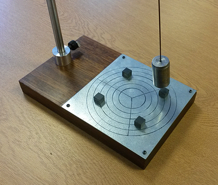
demonstration of the magnetic pendulum — Figure 1: The magnetic pendulum: a great demonstration rolled-out during open days and in lectures (here, using four base-plane magnets rather than three).

The objective of this article is to consider the pendulum problem and to illustrate how some of its inherent complexity can be visualised and understood through the prism of dynamical systems [3]. Our approach to formulating a phenomenological model will largely follow Peitgen, Jürgens and Saupe [4]; it involves a blend of classical mechanics with a slightly revised formulation for magnetic interactions, and we consider the case of four base-plane magnets rather than three.

A toy equation

To capture the essence of the dynamics, any physical model must account for three main ingredients: the pendulum’s free swing, dissipation (e.g., due to air resistance) and the interaction between the bob and base-plane magnets. We proceed by placing the four magnets at unit distance from the origin of the $(x,y)$ plane so that they sit on the corners of a square (see Figure 1). In three-dimensional (3D) space, the bob moves along the lower surface of a sphere whose centre coincides with the suspension point and whose radius is equal to the length of the string. However, numerical integration of the spherical-pendulum equations of motion is fraught with computational headaches [5]. Instead, we adopt a plan view of the system by looking down directly onto the $(x,y)$ plane so that the projection of the bob’s position is given by the vector $\textbf{x}(t) \equiv (x(t),y(t))$ at time $t$ .

In this reduced geometry, gravity supplies a torque that tends to pull the bob back to its straight-down position above the centre of the square, $\textbf{x} = \textbf{0}$ . If the string is much longer than typical $x$ and $y$ displacements, then the small-angle approximation may be safely deployed [6]. In so doing, the gravitational restoring force is modelled by $\textbf{F}_{\text{grav}} \propto -\textbf{x}$ , and we choose units so that the constant of proportionality may be set to one.

Lumped losses are accommodated by anticipating that damping is proportional to speed and hence $\textbf{F}_{\text{losses}} = -b\dot{\textbf{x}}$ , where $\dot{\textbf{x}} \equiv {\rm d}\textbf{x}/{\rm d} t$ and $b > 0$ is the dimensionless loss coefficient.

Magnetism is enormously complicated and it is not unreasonable to assert that a complete understanding of magnetic phenomena eludes physics even today. As testament, only relatively recently has a formula been derived to quantify the force between two small magnetic dipoles [7]. The magnitude of that force is predicted to vary as $1/\operatorname{distance}^4$ rather than $1/\operatorname{distance}^2$ [4, 6]. Compare that surprising situation to Coulomb’s law of electrostatics, where the inverse-square relation for point charges (electric monopoles) has been known for nearly two and a half centuries.

It is now instructive to combine the effects of gravity and magnetism into a potential energy function $V(\textbf{x}) = |\textbf{x}|^2/2 + V_{\textrm{mag}}(\textbf{x})$ , where

(1) $\begin{equation*} V_{\operatorname{mag}}(\textbf{x}) \equiv -\frac{1}{3}\sum_{n = 1}^4\frac{p_n}{(|\textbf{X}_n - \textbf{x}|^2 + h^2)^{3/2}} + V_0. \end{equation*}$

The first term in $V$ is the standard paraboloid associated with an isotropic linear restoring force, while $V_{\operatorname{mag}}$ sums over $1/{\operatorname{distance}}^3$ potentials centred on base-plane positions $\textbf{x} = \textbf{X}_n$ (the constant $V_0$ is added simply to ensure that the potential-energy minimum is always $V = 0$ ). The set of numbers $\{p_n\}$ determine the polarity of the constituent base-plane magnets relative to the bob: $p_n = +1$ corresponds to the attraction of opposite poles and $p_n = -1$ to the repulsion of like poles (see Figure 2). Singular forces that would result as $\textbf{x} \rightarrow \textbf{X}_n$ are suppressed by introducing a parameter $h$ , which might be interpreted physically as the dimensionless average height of the bob above the base plane [6]. We have set $h = 1/2$ throughout, for definiteness.

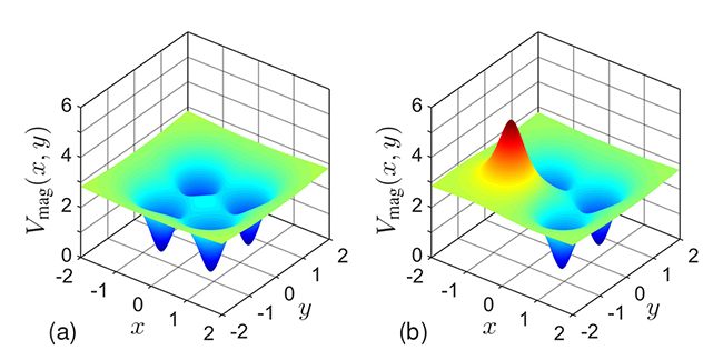
Figure 2: Contribution to the potential energy surface from magnetic interactions: (a) The base-plane magnets are all in the opposite-poles-attract configuration $(\bm{p_1 = p_2 = p_3 = p_4 = + 1})$ relative to the bob, which then sees four valleys; (b) Magnet 3 is flipped to be in the like-poles-repel configuration $(\bm{p_3 =-1})$ so that the bob experiences a potential hill.

The equation of motion is now $\ddot{\textbf{x}} = -b\dot{\textbf{x}} - \nabla V(\textbf{x})$ , where $\nabla$ denotes the spatial gradient operator. More explicitly,

(2) $\begin{equation*} \ddot{\textbf{x}}(t) + b\dot{\textbf{x}}(t) + \textbf{x}(t) = \sum_{n=1}^4p_n\frac{\textbf{X}_n - \textbf{x}(t)}{\left(|\textbf{X}_n - \textbf{x}(t)|^2+h^2\right)^{5/2}}. \end{equation*}$

Equation (2) does a superb job of mimicking the complex dynamics observed in any demonstration of a magnetic pendulum. The left-hand side is just a damped simple-harmonic oscillator moving in 2D while the right-hand side accounts for pairwise magnetic interactions and provides a coupling between otherwise-independent motions along the $x$ and $y$ directions. It is the interplay between these dissipative and nonlinear feedback loops that facilitates the emergence and richness of deterministic chaos (note that our model contains no trace of randomness!).

Fixed points and their stability

For arbitrary initial data $\textbf{x}(0)$ and $\dot{\textbf{x}}(0)$ , we expect the pendulum to come to rest as $t\rightarrow\infty$ because damping smoothly and continuously drains kinetic energy out of the motion. These equilibrium solutions, denoted by $\textbf{x}_\textrm{eq}$ , are associated with zero velocity ( $\dot{\textbf{x}}_\textrm{eq} = \textbf{0}$ , a state of rest) and zero acceleration ( $\ddot{\textbf{x}}_\textrm{eq} = \textbf{0}$ , experiencing no net force). From Equation (2), it follows that $\textbf{x}_{\operatorname{eq}}$ must satisfy

(3) $\begin{equation*} \textbf{x}_{\operatorname{eq}} - \sum_{n = 1}^4p_n\frac{\textbf{X}_n - \textbf{x}_{\operatorname{eq}}}{\left(|\textbf{X}_n - \textbf{x}_{\operatorname{eq}}|^2 + h^2\right)^{5/2}} = \textbf{0}, \end{equation*}$

and it is worth spending some time thinking about what this equation means in physical terms.

Inspection of Figure 2 leads us to expect that Equation (3) should probably have up to five acceptable roots. A base-plane magnet in the opposite-poles-attract configuration, say magnet $m$ and with $p_m = +1$ , typically gives rise to an absolute minimum in the potential energy surface. However, the precise location of that minimum is not at $\textbf{x}_{\operatorname{eq}} = \textbf{X}_m$ , as one might first suppose. Rather, it is at some other nearby position determined by physics (namely, where the net forces due to gravity and all the competing magnetic interactions balance one another exactly).

When all the base-plane magnets have $p_n = + 1$ for $n = 1, \dots, 4$ , symmetry demands that there exist four $\textbf{x}_{\operatorname{eq}}$ values lying at the same angular positions as $\left\{\textbf{X}_n\right\}$ but displaced slightly towards the origin in the radial direction. Any evolving $\textbf{x}(t)$ is then pulled towards these four unique fixed-point attractors in the $(x,y)$ plane. Such points are stable since they correspond to potential-energy minima: small disturbances tend to result in vibrations that diminish as $t \rightarrow \infty$ , with the pendulum relaxing back to its stationary state.

Potential-energy maxima tend to characterise like-poles-repel configurations. Such points are unstable and may be classified as repellors since they are associated with repulsive forces. That is not to say that the pendulum cannot stop at potential maxima; such an outcome is just extremely unlikely since any vanishingly small perturbation (such as from a slight table wobble) destroys the unstable equilibrium state. We also note that the origin of the $(x,y)$ plane may or may not be an equilibrium point, depending upon the choice of $\left\{p_n\right\}$ . When all four magnetic interactions are attractive, $\textbf{x}_{\operatorname{eq}} = \textbf{0}$ corresponds to an unstable maximum: any disturbance to $\textbf{x}_{\operatorname{eq}} = \textbf{0}$ tends to result in trajectories that diverge and ultimately stop at one of the other attracting magnets.

Basins of attraction

To proceed, we consider first the release from rest initial-value problem (IVP) and when all the magnetic interactions are attractive. The displacement of the bob at time zero, denoted by $\textbf{x}(0) \equiv (x_0,y_0)$ , is freely adjustable but its velocity is always set to zero, $\dot{\textbf{x}}(0) \equiv (\dot{x}_0,\dot{y}_0) = (0,0)$ . A desired section of the $(x_0,y_0)$ plane is then represented by a grid of points, and Equation (2) integrated systematically for every initial condition $(x_0,y_0)$ contained within that section. The winning magnet from each calculation is recorded, and the results are colour-coded and then overlayed on top of the $(x_0,y_0)$ plane.

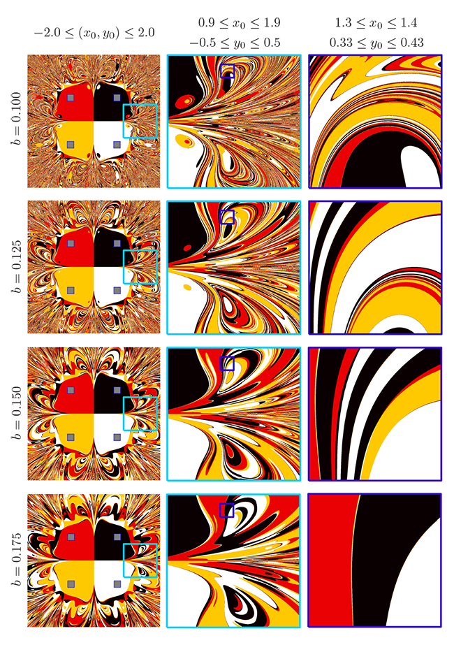
In Figure 3, the set of all initial conditions whose subsequent trajectories converge on magnet 1 is shown in black; that collection of black points is the basin of attraction for magnet 1 [8]. Similarly colour-coded results apply for the other magnets 2 (red), 3 (yellow) and 4 (white), but the colour provides no information about the path taken from a start point to its corresponding end point. Alternatively, one might consider the impulsive IVP by fixing the starting position at an equilibrium point such as $\textbf{x}(0) = \textbf{0}$ and applying an impulse in a particular direction. Such an impulse can be controlled by specifying the components of the initial velocity $\dot{\textbf{x}}(0)$ , and the patterns that emerge in the $(\dot{x}_0,\dot{y}_0)$ plane are similar to those given in Figure 3.

The basins of attraction emerging from both IVPs have some fascinating properties. Whether in real space [the $(x_0,y_0)$ plane] or velocity space [the $(\dot{x}_0,\dot{y}_0)$ plane], the basin patterns have the same symmetries as a square (four reflections and four rotations). Much of that symmetry is lost when, say, magnet 3 is flipped by setting $p_3 = -1$ . The potential around $\textbf{X}_3$ becomes a hill instead of a valley (see Figure 2), and the magnetic interaction is, thus, always repulsive in that neighbourhood. We then find the basins have the same symmetry as an isosceles triangle (a single reflection in the line $y_0 = x_0$ and no rotations; see Figure 4).

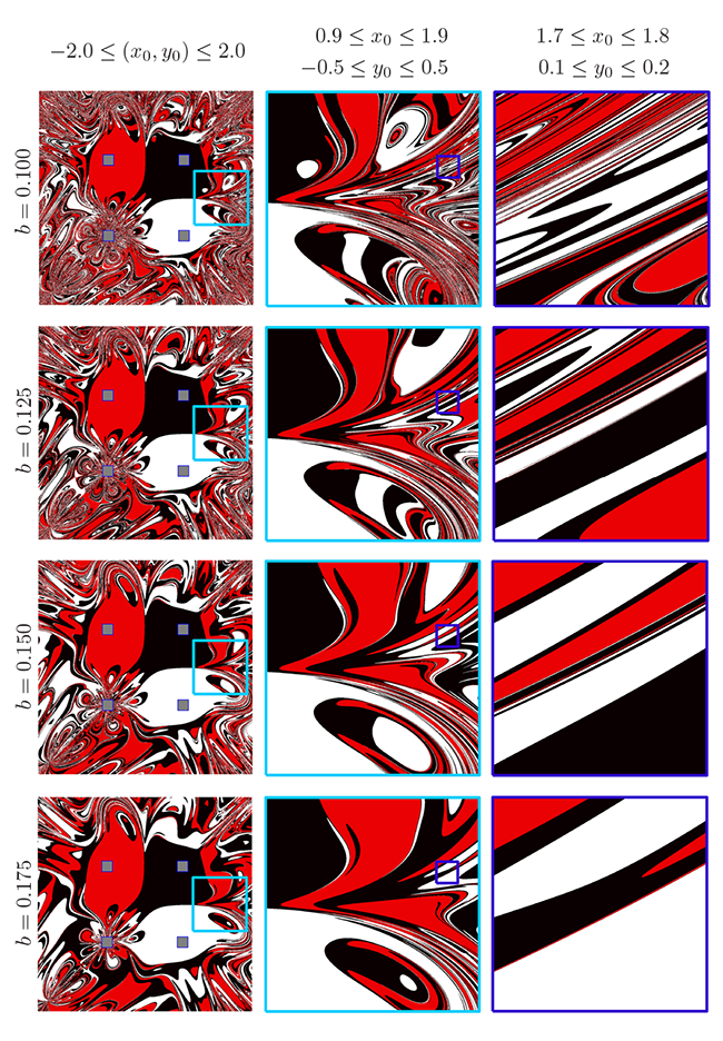
Basins of attraction magnet 3 repels — Figure 4: Basins of attraction in real space when base-plane magnet 3 is flipped so that it repels the bob. Note also the butterfly escaping from magnet 3.

Another feature of the basins is that, while they clearly make very striking intertwined patterns, an increasing level of dissipation tends to decrease the density of the pattern substructure. Moreover, the boundaries between adjacent colours are examples of fractals: that is, patterns exhibiting some degree of self-similarity (which may be exact or statistical) under magnification.

More subtly, a solid interface between any two colours never quite forms; the other two colours are always tightly packed in. For instance, in Figure 3 one cannot jump from red to yellow without also jumping across black and white [9].

Uncertainty and unpredictability

As a way to quantify the susceptibility of the pendulum to initial fluctuations, we deploy the method developed by Grebogi et al. [2] in their pioneering analysis of FSS. For each initial condition $\textbf{x}_0 \equiv (x_0,y_0)$ , two other related starting points are also considered: typically $\textbf{x}_{0 +\epsilon} \equiv (x_0 + \epsilon,y_0)$ and $\textbf{x}_{0-\epsilon} \equiv (x_0 - \epsilon,y_0)$ . The small positive number $\epsilon \ll \mathcal{O}(1)$ might be interpreted either as a formal perturbation to the pendulum’s input or as the radius of a disc of uncertainty representing a finite limit on experimental precision. If $\textbf{x}_0$ , $\textbf{x}_{0 + \epsilon}$ and $\textbf{x}_{0-\epsilon}$ all give rise to trajectories that converge to the same magnet, then $\textbf{x}_0$ does not possess FSS (see Figure 5).

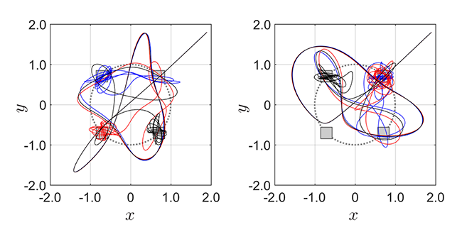
Figure 5: Trajectories on the potential energy surfaces shown in Figure 2. The unperturbed initial displacement is chosen to be $\bm{\textbf{x}_0 \equiv (x_0,y_0) = (1.9,1.8)}$ and the pendulum is released from rest. Subsequent motions are shown for $\bm{\textbf{x}(0)}$ set to $\bm{\textbf{x}_0}$ (black curves), $\bm{\textbf{x}_{0 + \epsilon}}$ (blue) and $\bm{\textbf{x}_{0-\epsilon}}$ (red) when $\bm{\epsilon = 10^{-3}}$ .

Consider a domain of initial conditions, $\Gamma$ , comprising a total of $N_\Gamma$ points and with $N_\epsilon$ of them susceptible to FSS. Many systems follow a power-law relation $N_\epsilon/N_\Gamma \equiv f_\epsilon \sim \epsilon^\alpha$ , where $0 < \alpha < 1$ is the uncertainty exponent. When $\Gamma$ is a 2D domain (such as we have here), one typically defines $\alpha \equiv 2 - D$ , with $D$ being known as the uncertainty dimension. After a back-of-the-envelope calculation, one finds

(4) $\begin{equation*} D = 2 - \frac{\textrm{d}\log_{10}(f_\epsilon)}{\textrm{d}[\log_{10}(\epsilon)]} \end{equation*}$

and that $1 < D < 2$ . Greater sensitivity to fluctuations at the input is associated with smaller $\alpha$ exponents and thus, with $D$ values that tend toward 2. Thus, in quite an elegant way, the degree of FSS exhibited by a system can be directly related to the level of pattern complexity in its basin boundaries. In contrast, boundaries that are regular (i.e., non-fractal) are characterised by $\alpha = 1$ .

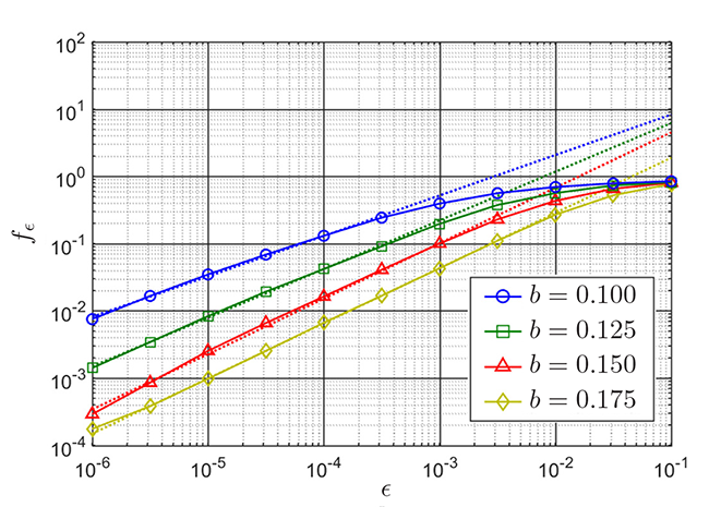
Figure 6: Numerical calculation of the log–log spectra computed for the basin patterns shown in the centre panes of Figure 3. Estimated values of the uncertainty dimension $\bm{D}$ are obtained by fitting curves: $\bm{D\approx1.40}$ $(\bm{b = 0.100}),$ $\bm{D\approx1.28}$ $(\bm{b = 0.125})$ and $\bm{D\approx1.18}$ $(\bm{b = 0.150}$ and $\bm{b = 0.175})$ .

Figure 6 shows the log–log spectra computed for the basins of attraction given in the centre panes of Figure 3. In the small $\epsilon$ regime, the curves are very nearly linear with the property that $D$ decreases with increasing $b$ . This result makes physical sense and agrees with what we might conclude just from a qualitative inspection: stronger dissipation appears to reduce overall pattern complexity. Such a reduction is manifest mathematically as a lowering of the uncertainty dimension, which ranges from $D \approx 1.40$ at low $b$ to $D \approx 1.18$ at high $b$ .

Towards larger $\epsilon$ regimes, the log–log spectra gradually flatten out. It follows that $D$ is greater in these regions, providing some evidence that the density of pattern detail in the magnetic-pendulum basin boundaries is an inherent function of scale (structures with this property are sometimes classified generically as scale-dependent fractals). Similar trends in behaviour are also found for the patterns in the central panes of Figure 4.

Concluding remarks

We have gone beyond the standard equilateral-triangle incarnation of the magnetic pendulum [4, 6], implemented a more physical model of magnetic interactions [7], experimented with polarity, computed basins of attraction and explored susceptibility to initial fluctuations by estimating fractal dimension. In other words, we have had enormous fun playing with a purely deterministic toy equation, which, despite all its simplifications, remains a highly nonlinear problem in the 4D $(x,y,\dot{x},\dot{y})$ phase space [5].

The phenomenon of sensitive dependence on initial conditions appears ubiquitously throughout Nature, and it is far more pervasive than one might first recognise. It turns out to be a key feature of almost every system that has competing feedback loops [3], even highly simplified models such as Equation (2). More profoundly, the relationship between final state sensitivity and the mathematics of fractal dimension, as discovered by Grebogi et al. [2] over three decades ago, appears to be deeply embedded within physical law.

The magnetic pendulum really is a paradigm of unpredictability, and there is almost no limit to the curiosity-driven variations one might try. The magical quality of its motion is also a very powerful tool for outreach purposes and in appealing to the imagination, especially when experimental demonstrations are accompanied by computer visualisations. Audiences – whether they are prospective students at open days, undergraduates in lectures or enthusiasts at MathsJam gatherings – are invariably mesmerised by the hypnotic motion of the swinging bob and its uncertain destination. As a device for piquing interest in physics and mathematics, is there anything better?

James M. Christian CMath FIMA and Holly A. J. Middleton-Spencer
University of Salford

References

Lorenz, E.N. (1972) Predictability; does the flap of a butterfly’s wings in Brazil set off a tornado in Texas? American Association for the Advancement of Science, 139th Meeting.
Grebogi, C., McDonald, S.W., Ott, E. and Yorke, J.A. (1983) Final state sensitivity: an obstruction to predictability, Phys. Lett., vol. 99, pp. 415–418.
Alligood, K.T., Sauer, T.D. and Yorke, J.A. (2000) Chaos: An Introduction to Dynamical Systems, Springer.
Peitgen, H.-O., Jürgens, H. and Saupe, D. (1992) Chaos and Fractals: New Frontiers of Science, Springer.
Kana, D.D. and Fox, D.J. (1995) Distinguishing the transition to chaos in a spherical pendulum, Chaos, vol. 5, pp. 298–310.
Motter, A.E., Gruiz, M., Károlyi, G. and Tél, T. (2013) Doubly transient chaos: generic form of chaos in autonomous dissipative systems, Phys. Rev. Lett., vol. 111, no. 194101.
Yung, K.W., Landecker, P.B. and Villani, D.D. (1998) An analytical solution for the force between two magnetic dipoles, Mag. Elec. Sep., vol. 9, pp. 39–52.
Nusse, H.E. and Yorke, J.A. (1996) Basins of attraction, Science, vol. 271, pp. 1376–1380.
Daza, A., Wagemakers, A., Sanjuán, M.A.F. and Yorke, J.A. (2015) Testing for basins of Wada, Sci. Rep., vol. 5, no. 16579.