The good old days
I would not class myself as old but, equally, I can no longer claim to be in the first flush of youth. And, whilst I am not always the most observant of people, I have managed to spot some of the trends that have occurred during my lifetime. If our younger readers will forgive the trip down memory lane, I remember the advent of the Sony Walkman or, more generically, the portable, personal music player – although many passengers on public transport may take issue with my use of the word ‘personal’.
Of course, in that case, music came on cassette tapes. By modern standards, this constrained the amount of music that could be listened to (and carried on one’s person). In my day, the standard was a 90-minute tape, 45 minutes on each side. Whilst theoretically possible, finding a particular song within that 45 minutes was practically very difficult. So, at least in my case, music was listened to sequentially, in the order that the artist intended.
Nowadays, with digital formats and modern devices, you can carry around almost endless amounts of music (and video). You can also call up any track as and when you desire, assuming you can remember that you have it, of course. You can even create your own playlists, choosing which tracks come in which order.
I am not a music critic and I do not understand enough about people and their behaviour, to say how these changes have affected people and their listening habits, but, it seems to me, that the move from analogue-to-digital music storage is part of a much wider trend. Indeed, you could say that the past decades have seen the rise of the digital.
Computation
Currently, computation is mainly a digital endeavour, but this was not always the case. For example, the Antikythera mechanism dates from around the second century BCE. This mechanical (or analogue) computer tracks the cycles of the Solar System. Given the importance of computing to our lives, it is perhaps not surprising that there are modern implementations of analogue computation, including chemical reaction networks (CRNs).
In simple terms, a CRN operates over a finite set of species,  . In that context, a reaction is a tuple:
  , with
  being reactants,
  being products and
  being rates. A collection of one or more reactions, over the same set of species, is a CRN.
As an example, consider the following single-reaction CRN:
(1) ![\begin{equation*} X_1 + X_2 \xrightarrow[]{1} Y. \end{equation*}](https://ima.org.uk/wp/wp-content/ql-cache/quicklatex.com-0de41b88900522b847f9830a1d5fd0ce_l3.svg "Rendered by QuickLaTeX.com")
This has three species:  and
and  are reactants, and
  is a product. The rate is indicated by the number above the arrow. For simplicity, if the rate is not indicated, it is assumed to be unity.
An idealised implementation of this CRN is shown in Figure 1. We begin with slightly less of than and no . Over time, the reaction progresses so that all of the (and most of the ) is converted into .
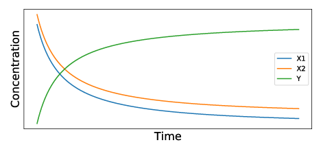
There are several ways that we can view this system. As described above, the system implements  . Alternatively, we can view the initial states of and as encoding a high signal, in which case we have implemented an
  gate. Depending on our motivation, either of these may be more natural: if we are trying to represent a system then finding the minimum of two values may be useful; or, if we are trying to encode a logic circuit in a CRN, then logic gates are required.
Polynomial equations
We can also use CRNs to solve equations or, equivalently, to calculate algebraic numbers. Consider the polynomial equation  given by:

We assume that  , using
  if this is not the case, and construct a CRN that finds the smallest positive root of this equation. Furthermore, we will do this using only one species. The construction uses the following rules:
![\begin{equation*} \begin{split} \text{If } c_k > 0 & \text{ add } kX \xrightarrow[]{c_k} \left( k + 1 \right)X, \\ \text{If } c_k < 0 & \text{ add } kX \xrightarrow[]{|c_k|} \left( k - 1 \right)X. \end{split} \end{equation*}](https://ima.org.uk/wp/wp-content/ql-cache/quicklatex.com-1597958bf8bba40ab952bbe16c4bd581_l3.svg "Rendered by QuickLaTeX.com")
To make this concrete, consider  with
with  ,
,  and
and  . Hence, we need these reactions:
(2) ![\begin{equation*} \begin{split} \emptyset \xrightarrow[]{2} X, & \qquad \left[ c_0 \right] \\ 2X \xrightarrow[]{1} X. & \qquad \left[ c_2 \right] \end{split} \end{equation*}](https://ima.org.uk/wp/wp-content/ql-cache/quicklatex.com-60b72855f637a28fe4599f26988e9a8d_l3.svg "Rendered by QuickLaTeX.com")
Note that, the first reaction begins with the empty set. That is,  is apparently created out of nothing. We will briefly return to this topic later. For the moment, assume that this is, in some way, possible. The results of an idealised implementation of this system are shown in Figure 2. It is apparent that, over time, reaches the correct value (shown by the dashed line).
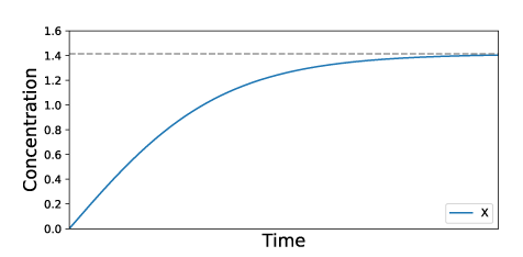
To provide an intuitive understanding of why this is the case, we consider the link between CRNs and ordinary differential equations (ODEs). In particular, we link species with quantity  and consider the evolution of this quantity with time. Each reaction contributes to this evolution as shown below:
![\begin{equation*} \label{eqn:polyproof} \begin{split} kX \xrightarrow[]{c_k} \left( k + 1 \right)X, & \qquad \frac{\textrm{d} x}{\textrm{d} t} = c_k x^k, \\ kX \xrightarrow[]{|c_k|} \left( k - 1 \right)X, & \qquad \frac{\textrm{d} x}{\textrm{d} t} = -|c_k| x^k. \end{split} \end{equation*}](https://ima.org.uk/wp/wp-content/ql-cache/quicklatex.com-b478323b52ceb68b8290fa1485e746c0_l3.svg "Rendered by QuickLaTeX.com")
Given the above, it is apparent that the CRN dynamics satisfy  . We start with
  and, since we have guaranteed
  , we know that must begin to increase. When reaches the first positive root of
  , we have, by construction,
  . So, remains at that constant value.
Trigonometric functions
CRNs can also be used to calculate trigonometric functions. The reactions to calculate  are shown in (3). The output from an idealised implementation is illustrated in Figure 3.
(3) ![\begin{equation*} \begin{split} F_M & \xrightarrow[]{1} F_M + Z_P, \\ F_P & \xrightarrow[]{1} F_P + Z_M, \\ Z_P & \xrightarrow[]{1} Z_P + F_P, \\ Z_M & \xrightarrow[]{1} Z_M + F_M, \\ F_M + F_P & \xrightarrow[]{1000} \emptyset, \\ Z_M + Z_P & \xrightarrow[]{1000} \emptyset. \end{split} \end{equation*}](https://ima.org.uk/wp/wp-content/ql-cache/quicklatex.com-7b4ebb47758d61a786d0d30091dffb3d_l3.svg "Rendered by QuickLaTeX.com")
As this example illustrates, working with CRNs, even in their idealised form, can be complicated. In particular, when working with CRNs, we measure the concentration of a species, which, by definition, is a positive value. Conversely, covers the range ![{\left[ -1 , +1 \right]}](https://ima.org.uk/wp/wp-content/ql-cache/quicklatex.com-c66a79e68405e9807ec7dbc08ab94755_l3.svg "Rendered by QuickLaTeX.com") . To account for this, Equation (3) has two output species,
. To account for this, Equation (3) has two output species,  and
and  . The first of these covers the positive part of the range, the latter covers the negative part (multiplied by
  ). Equivalently, our desired output is given by
  .
.
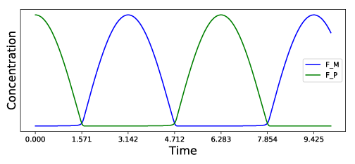
The last two reactions in Equation (3) are annihilation reactions, which act to ensure one of and always remains small (and similarly for  and
and  ). The faster the rate of these annihilation equations, the neater the handover between and . Close observation of Figure 3 suggests, that even in our idealised situation, this handover is noticeably imperfect, so a rate greater than 1 000 would probably be preferable.
To understand why the CRN in Equation (3) produces , we note that the six reactions result in the following ODEs:
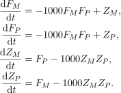
It follows that  . More generally, we have created a system that, for a general function
  , satisfies
  . This, together with an appropriate initialisation condition at time zero, delivers us . Obviously, a different initialisation condition would yield
  .
.
Dynamical systems
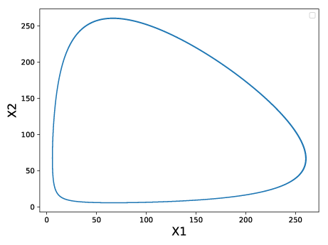
Previous discussions have focused on the link between CRNs and ODEs. Given this link, it is natural to use CRNs to represent dynamical systems, for example the Lotka–Volterra predator–prey model. In this case, our reactions (using as prey and as predator) are
(4) ![\begin{equation*} \begin{split} X_1 + X_2 & \xrightarrow[]{0.00005} 2 X_2, \\ X_1 & \xrightarrow[]{0.0033} 2 X_1, \\ X_2 & \xrightarrow[]{0.0033} \emptyset. \\ \end{split} \end{equation*}](https://ima.org.uk/wp/wp-content/ql-cache/quicklatex.com-6594f2c7b330ec98a2697b815e9e46b5_l3.svg "Rendered by QuickLaTeX.com")
For completeness, the phase plot resulting from an idealised implementation is shown in Figure 4.
Despite their obvious link to CRNs, there are some ODEs that cannot easily be implemented in this manner. As an example, consider the Lorenz attractor, which has three variables (,  and
and  ) governed by three parameters (
 ,
,  and
and  ) and the following equations:
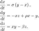
In this case, it seems there is no easy way to achieve the  term in
  . This is because species are only consumed (that is, their quantity reduces, and their time derivative is negative) if they are reactants in an equation. In that case, the speed of the reaction is influenced by the concentration of the relevant species. So, the species itself has to appear in a negative term. Hence, whilst we could (in ) easily create a term
  , we cannot easily create a term . There are ways of transforming ODEs to produce CRNs that exhibit similar kinetics, so a CRN can model the Lorenz attractor, but their consideration is outside the scope of this article.
Implementation details
The previous discussions have, hopefully, illustrated some of the interesting features of CRNs as a computing medium. We have shown they are able to model logic gates, to solve equations (and calculate algebraic numbers), to represent trigonometric functions and to model dynamical systems. In addition, as a review of the literature shows, amongst other things, they are capable of playing rock-paper-scissors and implementing neural networks. More particularly, they represent a Turing complete computational system.
However, we have repeatedly stressed the notion of an idealised implementation. We have also allowed species to be created from nothing, for example in (2). These considerations prompt the question: can CRNs be implemented in practice? If so, how easy is this?
Apparently, one way this may be achieved is through DNA strand displacement (DSD) or, more formally, toehold-mediated branch migration and strand displacement. I readily admit that the full details of this process are beyond my area of expertise; to be honest, the same could be said of the basic details of the process as well. However, the literature describes a number of schemes that can compile from CRN to DSD. In some cases the equivalence between the theoretical (CRN) and implemented (DSD) mechanisms can be proven; in other cases it cannot.
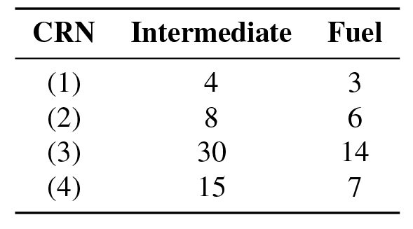
These schemes extend the types of species. In addition to reactants and products (used above, and more generally termed signal species), there are also intermediate species and fuel species. In simple terms, the former break the idealised reactions into physically implementable steps, whilst the latter catalyse reactions and control the sequence of execution. Table 1 shows the number of such species used in the CRNs described above.
Of course, it would be unrealistic to expect actual DNA-based implementations to behave in exactly the same way as the idealised representations (based on ODEs) illustrated above. In reality, the biological system will involve large numbers of molecules, which will interact in a stochastic fashion. Hence, a key consideration of CRNs is their robustness: for example, the system created in the polynomial root-finding example is such that the calculated (smallest positive) root is an exponentially stable point in the ODE-defined system.
There are other challenges as well. For example, DNA-based implementations of CRNs tend to calculate an answer over a relatively long period (for example, hours).
The good new days
CRNs and DNA-based computing are not going to replace traditional digital forms. Despite that, they are interesting for a number of reasons. For example, they provide a different way of looking at computation-related problems and, in my experience, different ways of looking at things often lead to insights.
More importantly, when encoded using DNA strands, a program has a physical structure. Rather than using a program to control a device that interacts with the real world, that interaction can happen directly with the program itself. This opens up huge possibilities, including nanoscale engineering and the use of DNA-based nanostructures as drug delivery carriers.
Whilst the rise of the digital has brought many benefits, CRNs (and DNA-based computing) demonstrate there are still areas where analogue approaches have great value. Hence, personally speaking, I am very much looking forward to some ‘good new days’ where the analogue and the digital combine so we can have, to quote Hannah Montana (who sounds great regardless of medium), ‘the best of both worlds’!
Rob Ashmore CMath CSci FIMA
Dstl
Sources
Details of the Antikythera mechanism are available from The Antikythera Mechanism Research Project. Compilation from CRNs to DSD and the simulations of idealised behaviours were achieved using the Nuskell compiler. This includes a number of different CRN-to-DSD compilation schemes.
The polynomial root-finding example is taken from [1]. The cosine function is based on an example in [2]. The Lotka–Volterra model is taken from [3].
Acknowledgement
‘Urban Maths’ cartoonist: Adrian Metcalfe
The views and opinions expressed herein are those of the author and do not necessarily reflect those of Dstl.
Crown Copyright © 2020 Dstl. This information is licensed under the Open Government Licence v3.
References
- Huang, X. et al. (2019) Real-time computability of real numbers by chemical reaction networks, Nat. Comput., vol. 18, no. 1, pp. 63–73.
- Fages, F. et al. (2017) Strong Turing completeness of continuous chemical reaction networks and compilation of mixed analog–digital programs, CMSB 2017, 15th Int. Conf. Computational Methods in Systems Biology, Darmstadt, Germany, pp. 108–127.
- Soloveichik, D. et al. (2010) DNA as a universal substrate for chemical kinetics, Proc. Natl. Acad. Sci. USA, vol. 107, no. 12, pp. 5393–5398.
Reproduced from Mathematics Today, June 2020
Download the article, Urban Maths: The Best of Both Worlds (pdf)