Unscrambling the Infinite: Can we Compute Spectra?
Matthew Colbrook was awarded the 2021 IMA Lighthill–Thwaites Prize at the British Applied Mathematics Colloquium (BAMC), ‘for his simply explained ground-breaking computational work’.
When you listen to a piece of music, the sound signal consists of a sum of individual simple frequencies or oscillatory components. Mathematically, these different components can be revealed by applying the Fourier transform, named after the French mathematician Joseph Fourier. Fourier introduced the idea of representing temperature as a sum of simpler oscillatory components in his fundamental study of heat. This representation allowed the system to be split into simpler parts and analysed. [latexpage]
More generally, this idea of decomposition or diagonalisation is applied to linear operators, a type of mathematical mapping that permeates mathematical analysis and applications. Just as a sound signal can be broken down into a set of simple frequencies, an operator can be decomposed into simple constituent parts via its ‘spectrum’.
Nowadays, spectral theory is ubiquitously used throughout the sciences to solve complex problems. For systems described by a finite number of parameters, this problem is mathematically equivalent to finding the zeroes of a polynomial. In general, the problem can only be solved computationally, thanks to the insolvability of the quintic.$^1$ Here, the most famous algorithm is the QR algorithm [1], hailed as one of the ten algorithms with the most significant influence on science, numerical analysis and engineering in the 20th century [2]. However, often the problems encountered involve an infinite number of parameters or coordinates – they are infinite-dimensional, typically leading to an infinite spectrum.$^2$
Famous examples of spectral theory include the energy levels of systems in quantum mechanics, partial differential equations (equations measuring rates of change), vibrations in structure analysis, studying fluid stability, describing transmission in wave and acoustic problems. Due to the continual advance in computing and the desire for realistic modelling in applications, the following question is fundamental: How do we approximate spectra for infinite-dimensional problems on a (necessarily) finite computer?
This problem has a rich history that dates back at least 60 years and involves a who’s who of leading mathematicians and physicists, with many triumphs for computational mathematics and theoretical physics.
Yet, in general, spectral computations in infinite dimensions have remained notoriously difficult. When we apply a computational method, fundamental challenges include (a) missing parts of the spectrum and (b) approximating points that we think are close to the spectrum but actually are not (this is known as ‘spectral pollution’). Overcoming these two issues in the general case is a long-standing problem in computational mathematics [3].
Even if we have a method that avoids these pitfalls, we are still left with the question of determining which parts of an approximation to trust. Ideally, not only do we wish to approximate spectra, but also compute ‘error bounds’ telling us how close our approximation is to the true solution. This makes computations reliable and useful in applications, and can also be used in areas of pure mathematics such as computer-assisted proofs [4].
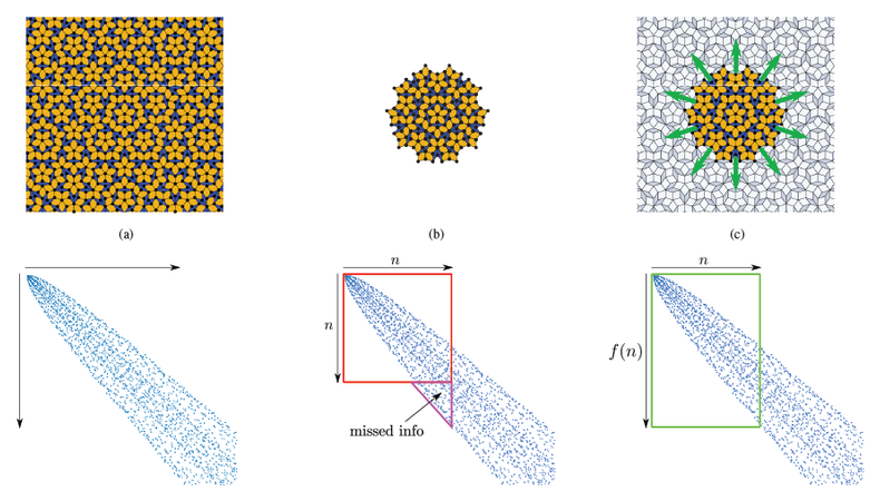
As an example of our resolution of the above question (see [5]), consider quasicrystals. Quasicrystals are non-repeating (aperiodic$^3$) structures with a long-range, self-similar nature (see Figure 1(a)). More generally, systems with long-range order and short-range disorder are abundant in nature.$^4$ Currently, aperiodic systems are not nearly as well understood as their periodic cousins.$^5$
We might ask, then: what are the physics of aperiodic systems? Understanding spectral properties is key to answering these types of questions. However, the aperiodic nature of quasicrystals, which makes them so interesting to study in the first place, also makes it a considerable challenge to approximate spectra associated with these systems!
We took a Penrose tile, a canonical model of a quasicrystal in 2D, and generated the lattice shown in Figure 1(a) by considering a lattice ‘site’ to exist at each vertex (the black dots) and tunnelling bonds along the edges of the tiles. The model taken is that of a charged particle, which can exist on the set of sites and can tunnel between the sites along the bonds. We then apply a perpendicular magnetic field, which modifies the tunnelling strengths to enforce the usual circular motion of a free charged particle in a magnetic field. The operator in this scenario is a Hamiltonian $H$ which, in matrix form, is given by
\[
(H\psi)_j=-\sum_{\langle j,k\rangle}\textrm{e}^{\textrm{i}\alpha_{kj}}\psi_k,
\]
with summation over sites connected by an edge. Here $\alpha_{kj}$ is a phase factor that is given in terms of the strength of the magnetic field and $\psi$ denotes the wave function.
The most common approach to computing spectra is to truncate the operator. Physically, in our example, this corresponds to truncating the tile and studying the interactions of a finite number of sites within the truncation (Figure 1(b)). Mathematically, this corresponds to studying a finite section of the operator and computing spectra of the corresponding finite-dimensional system (eigenvalues of finite square matrices shown as a red box in Figure 1).
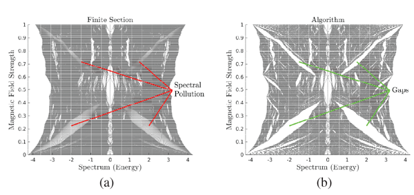
In this model, the dimension of this finite-dimensional system is precisely the number of sites included in the truncation. Figure 2(a) shows the output of this approach, where the approximation of the spectrum is plotted for different magnetic field strengths. We have labelled portions of this picture as ‘spectral pollution’ (recall the fundamental challenge (b) mentioned above, where points in the approximation have nothing to do with the true spectrum). This approach does not approximate the correct solution and does not provide any form of error bounds.$^6$
Instead, we truncate the operator differently [5]. Physically, in our example, we truncate the tile as before, but now also include the interactions of the finite truncation with the rest of the tile (Figure 1(c)). Mathematically, in this example, this method corresponds to studying a rectangular finite section/matrix of the operator (shown as a green box in Figure 1).
When written as a matrix, the Hamiltonian $H$ in this example is ‘sparse’, meaning it has finitely many non-zero entries in each column. For each site included in the truncation, the corresponding column of the matrix lists the interactions with other sites. The rectangular truncation simply includes the rows of the matrix with non-zero interactions. We can think of this as a tool for studying the full infinite-dimensional operator directly, even on a finite computer.
Leveraging this idea, we can now approximate spectra in such a way that (i) our approximations approach the correct solution as our truncation size increases (overcoming challenges (a) and (b) above), and (ii) such that we can explicitly bound the error of any computed approximation. The practitioner can now provide a desired error bound, which our algorithm will then adaptively realise.
Figure 2(b) shows the output of this approach for our example. We now (i) have the correct gaps in the spectrum, (ii) approximate the correct spectrum and, for this example, (iii) have a guaranteed error bound of 0.01. With this technique in hand, we can reliably probe the bulk physical properties of such aperiodic systems. Indeed, this technique is already allowing for the discovery and investigation of new physics in quasicrystalline systems, including their transport and topological properties.
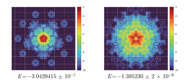
The above approach can be extended far beyond this example. Other types of operators that can be treated include non-local interactions (for readers familiar with the term, we can treat non-sparse matrices), partial differential equations and even non-Hermitian operators. The idea of treating operators directly can also be applied to other problems such as computing approximate states/eigenvectors (Figure 3), spectral projections and spectral measures$^7$ [6,7] and a whole zoo of spectral properties [8].
Going one step further, we can classify these problems in a computational hierarchy$^8$ [8]. This measures the intrinsic difficulty of computational problems and provides proofs of the optimality of algorithms, realising limits of what computers can achieve. For example, and rather surprisingly, computing spectra of operators similar to the above example is strictly easier than for compact operators,$^9$ which is itself easier than computing spectra of general self-adjoint operators.
Beyond spectral theory, this framework is now being applied to optimisation, machine learning and artificial intelligence, solving partial differential equations and computer-assisted proofs. As science and society become increasingly reliant on computations, it is essential to understand what is computationally possible and design algorithms that are optimal and achieve these bounds.
We hope that further studies of infinite-dimensional spectral computations will lead to advancements in this fascinating subject, as well as the foundations of computation in other areas of mathematics. We end with a fitting quotation from one of the heroes of spectral theory, David Hilbert (1925):
The infinite! No other question has ever moved so profoundly the spirit of humankind; no other idea has so fruitfully stimulated the intellect; yet no other concept stands in greater need of clarification.
Matthew Colbrook
University of Cambridge
Notes
This result, known as the Abel–Ruffini theorem, states that for degree higher than four, there is no formula for the zeroes of a general polynomial in terms of arithmetic operations and root extraction applied to the coefficients.
The name ‘spectral theory’ was first introduced by David Hilbert in his study of quadratic forms in infinitely many variables.
This means that shifting the structure by any finite distance, without rotation, cannot produce the same structure.
Fractals (structures that exhibit similar patterns at different scales) are another example.
The reason for this is not being able to apply a result known as Bloch’s theorem, which gives the form of solutions to Schrödinger’s equation with a periodic potential. For example, in a periodic crystal, the wave function can be decomposed as $\psi(\textbf{\mathrm{r}})=\textrm{e}^{\textrm{i}\textbf{\mathrm{k}}\cdot\textbf{\mathrm{r}}}p(\textbf{\mathrm{r}})$ for periodic function $p$ (with the same periodicity as the crystal). The ‘local’ approach discussed below circumvents the need for Bloch’s theorem or other results that rely on forms of symmetry.
For this particular model and method of finite section, states corresponding to spectral pollution are known as ‘edge states’. Physically, an important problem is to distinguish between these edge states and points that are in the spectrum of the full infinite tile.
One can think of spectral measures as describing the ‘shape’ of the operator. This is particularly important for operators with continuous spectra which, going back to the analogy of music, can be thought of as a continuum of frequencies.
This is the Solvability Complexity Index (SCI) hierarchy, which has roots in the work of Smale [9,10], and his programme on the foundations of computational mathematics and scientific computing, though it is quite distinct.
These are operators that, in their totality, can be approximated by finite-dimensional operators.
References
Francis, J.G.F. (1961) The QR Transformation Part 1, Comput. J, vol. 4, no. 3, pp. 265–271.
Dongarra, J. and Sullivan, F. (2000) Guest editors’ introduction: The top 10 algorithms, IEEE Ann. Hist. Comput., vol. 2, no. 1, pp. 22–23.
Arveson, W. (1994) The role of $C^*$-algebras in infinite dimensional numerical linear algebra, Contemp. Math., vol. 167, pp. 115–129.
Fefferman, C.L. and Seco, L.A. (1996) ‘Interval arithmetic in quantum mechanics’, in Kearfott, R.B. and Kreinovich, V. (eds.) Applications of interval computations, Springer US, pp. 145–167.
Colbrook, M.J., Roman, B. and Hansen, A.C. (2019) How to compute spectra with error control, Phys. Rev. Lett., vol. 122, no. 25, p. 250201.
Colbrook, M.J. (2021) Computing spectral measures and spectral types, Commun. Math. Phys., vol. 384, pp. 433–501.
Colbrook, M.J., Horning, A. and Townsend, A. (2021) Computing spectral measures of self-adjoint operators, SIAM Rev., to appear.
Colbrook, M.J. (2020) The Foundations of Infinite-Dimensional Spectral Computations, Doctoral dissertation, University of Cambridge.
Smale, S. (1981) The fundamental theorem of algebra and complexity theory, B. Am. Math. Soc., vol. 4, no. 1, pp. 1–36.
Smale, S. (1997) Complexity theory and numerical analysis, Acta Numer., vol. 6, pp. 523–551.

 As an example of our resolution of the above question (see [5]), consider quasicrystals. Quasicrystals are non-repeating (aperiodic$^3$) structures with a long-range, self-similar nature (see Figure 1(a)). More generally, systems with long-range order and short-range disorder are abundant in nature.$^4$ Currently, aperiodic systems are not nearly as well understood as their periodic cousins.$^5$
We might ask, then: what are the physics of aperiodic systems? Understanding spectral properties is key to answering these types of questions. However, the aperiodic nature of quasicrystals, which makes them so interesting to study in the first place, also makes it a considerable challenge to approximate spectra associated with these systems!
We took a Penrose tile, a canonical model of a quasicrystal in 2D, and generated the lattice shown in Figure 1(a) by considering a lattice ‘site’ to exist at each vertex (the black dots) and tunnelling bonds along the edges of the tiles. The model taken is that of a charged particle, which can exist on the set of sites and can tunnel between the sites along the bonds. We then apply a perpendicular magnetic field, which modifies the tunnelling strengths to enforce the usual circular motion of a free charged particle in a magnetic field. The operator in this scenario is a Hamiltonian $H$ which, in matrix form, is given by
\[
(H\psi)_j=-\sum_{\langle j,k\rangle}\textrm{e}^{\textrm{i}\alpha_{kj}}\psi_k,
\]
with summation over sites connected by an edge. Here $\alpha_{kj}$ is a phase factor that is given in terms of the strength of the magnetic field and $\psi$ denotes the wave function.
The most common approach to computing spectra is to truncate the operator. Physically, in our example, this corresponds to truncating the tile and studying the interactions of a finite number of sites within the truncation (Figure 1(b)). Mathematically, this corresponds to studying a finite section of the operator and computing spectra of the corresponding finite-dimensional system (eigenvalues of finite square matrices shown as a red box in Figure 1).
In this model, the dimension of this finite-dimensional system is precisely the number of sites included in the truncation. Figure 2(a) shows the output of this approach, where the approximation of the spectrum is plotted for different magnetic field strengths. We have labelled portions of this picture as ‘spectral pollution’ (recall the fundamental challenge (b) mentioned above, where points in the approximation have nothing to do with the true spectrum). This approach does not approximate the correct solution and does not provide any form of error bounds.$^6$
As an example of our resolution of the above question (see [5]), consider quasicrystals. Quasicrystals are non-repeating (aperiodic$^3$) structures with a long-range, self-similar nature (see Figure 1(a)). More generally, systems with long-range order and short-range disorder are abundant in nature.$^4$ Currently, aperiodic systems are not nearly as well understood as their periodic cousins.$^5$
We might ask, then: what are the physics of aperiodic systems? Understanding spectral properties is key to answering these types of questions. However, the aperiodic nature of quasicrystals, which makes them so interesting to study in the first place, also makes it a considerable challenge to approximate spectra associated with these systems!
We took a Penrose tile, a canonical model of a quasicrystal in 2D, and generated the lattice shown in Figure 1(a) by considering a lattice ‘site’ to exist at each vertex (the black dots) and tunnelling bonds along the edges of the tiles. The model taken is that of a charged particle, which can exist on the set of sites and can tunnel between the sites along the bonds. We then apply a perpendicular magnetic field, which modifies the tunnelling strengths to enforce the usual circular motion of a free charged particle in a magnetic field. The operator in this scenario is a Hamiltonian $H$ which, in matrix form, is given by
\[
(H\psi)_j=-\sum_{\langle j,k\rangle}\textrm{e}^{\textrm{i}\alpha_{kj}}\psi_k,
\]
with summation over sites connected by an edge. Here $\alpha_{kj}$ is a phase factor that is given in terms of the strength of the magnetic field and $\psi$ denotes the wave function.
The most common approach to computing spectra is to truncate the operator. Physically, in our example, this corresponds to truncating the tile and studying the interactions of a finite number of sites within the truncation (Figure 1(b)). Mathematically, this corresponds to studying a finite section of the operator and computing spectra of the corresponding finite-dimensional system (eigenvalues of finite square matrices shown as a red box in Figure 1).
In this model, the dimension of this finite-dimensional system is precisely the number of sites included in the truncation. Figure 2(a) shows the output of this approach, where the approximation of the spectrum is plotted for different magnetic field strengths. We have labelled portions of this picture as ‘spectral pollution’ (recall the fundamental challenge (b) mentioned above, where points in the approximation have nothing to do with the true spectrum). This approach does not approximate the correct solution and does not provide any form of error bounds.$^6$
 Instead, we truncate the operator differently [5]. Physically, in our example, we truncate the tile as before, but now also include the interactions of the finite truncation with the rest of the tile (Figure 1(c)). Mathematically, in this example, this method corresponds to studying a rectangular finite section/matrix of the operator (shown as a green box in Figure 1).
When written as a matrix, the Hamiltonian $H$ in this example is ‘sparse’, meaning it has finitely many non-zero entries in each column. For each site included in the truncation, the corresponding column of the matrix lists the interactions with other sites. The rectangular truncation simply includes the rows of the matrix with non-zero interactions. We can think of this as a tool for studying the full infinite-dimensional operator directly, even on a finite computer.
Leveraging this idea, we can now approximate spectra in such a way that (i) our approximations approach the correct solution as our truncation size increases (overcoming challenges (a) and (b) above), and (ii) such that we can explicitly bound the error of any computed approximation. The practitioner can now provide a desired error bound, which our algorithm will then adaptively realise.
Figure 2(b) shows the output of this approach for our example. We now (i) have the correct gaps in the spectrum, (ii) approximate the correct spectrum and, for this example, (iii) have a guaranteed error bound of 0.01. With this technique in hand, we can reliably probe the bulk physical properties of such aperiodic systems. Indeed, this technique is already allowing for the discovery and investigation of new physics in quasicrystalline systems, including their transport and topological properties.
The above approach can be extended far beyond this example. Other types of operators that can be treated include non-local interactions (for readers familiar with the term, we can treat non-sparse matrices), partial differential equations and even non-Hermitian operators. The idea of treating operators directly can also be applied to other problems such as computing approximate states/eigenvectors (Figure 3), spectral projections and spectral measures$^7$ [6,7] and a whole zoo of spectral properties [8].
Instead, we truncate the operator differently [5]. Physically, in our example, we truncate the tile as before, but now also include the interactions of the finite truncation with the rest of the tile (Figure 1(c)). Mathematically, in this example, this method corresponds to studying a rectangular finite section/matrix of the operator (shown as a green box in Figure 1).
When written as a matrix, the Hamiltonian $H$ in this example is ‘sparse’, meaning it has finitely many non-zero entries in each column. For each site included in the truncation, the corresponding column of the matrix lists the interactions with other sites. The rectangular truncation simply includes the rows of the matrix with non-zero interactions. We can think of this as a tool for studying the full infinite-dimensional operator directly, even on a finite computer.
Leveraging this idea, we can now approximate spectra in such a way that (i) our approximations approach the correct solution as our truncation size increases (overcoming challenges (a) and (b) above), and (ii) such that we can explicitly bound the error of any computed approximation. The practitioner can now provide a desired error bound, which our algorithm will then adaptively realise.
Figure 2(b) shows the output of this approach for our example. We now (i) have the correct gaps in the spectrum, (ii) approximate the correct spectrum and, for this example, (iii) have a guaranteed error bound of 0.01. With this technique in hand, we can reliably probe the bulk physical properties of such aperiodic systems. Indeed, this technique is already allowing for the discovery and investigation of new physics in quasicrystalline systems, including their transport and topological properties.
The above approach can be extended far beyond this example. Other types of operators that can be treated include non-local interactions (for readers familiar with the term, we can treat non-sparse matrices), partial differential equations and even non-Hermitian operators. The idea of treating operators directly can also be applied to other problems such as computing approximate states/eigenvectors (Figure 3), spectral projections and spectral measures$^7$ [6,7] and a whole zoo of spectral properties [8].
 Going one step further, we can classify these problems in a computational hierarchy$^8$ [8]. This measures the intrinsic difficulty of computational problems and provides proofs of the optimality of algorithms, realising limits of what computers can achieve. For example, and rather surprisingly, computing spectra of operators similar to the above example is strictly easier than for compact operators,$^9$ which is itself easier than computing spectra of general self-adjoint operators.
Beyond spectral theory, this framework is now being applied to optimisation, machine learning and artificial intelligence, solving partial differential equations and computer-assisted proofs. As science and society become increasingly reliant on computations, it is essential to understand what is computationally possible and design algorithms that are optimal and achieve these bounds.
We hope that further studies of infinite-dimensional spectral computations will lead to advancements in this fascinating subject, as well as the foundations of computation in other areas of mathematics. We end with a fitting quotation from one of the heroes of spectral theory, David Hilbert (1925):
Going one step further, we can classify these problems in a computational hierarchy$^8$ [8]. This measures the intrinsic difficulty of computational problems and provides proofs of the optimality of algorithms, realising limits of what computers can achieve. For example, and rather surprisingly, computing spectra of operators similar to the above example is strictly easier than for compact operators,$^9$ which is itself easier than computing spectra of general self-adjoint operators.
Beyond spectral theory, this framework is now being applied to optimisation, machine learning and artificial intelligence, solving partial differential equations and computer-assisted proofs. As science and society become increasingly reliant on computations, it is essential to understand what is computationally possible and design algorithms that are optimal and achieve these bounds.
We hope that further studies of infinite-dimensional spectral computations will lead to advancements in this fascinating subject, as well as the foundations of computation in other areas of mathematics. We end with a fitting quotation from one of the heroes of spectral theory, David Hilbert (1925):