Domestic holidays in the UK offer a great opportunity to escape the everyday without the challenges of packing lists, airports and refilling miniature shampoo bottles! Furthermore, we have the chance to explore the extensive variety of British landscapes and their ecosystems.
While exploring the outdoors, particularly in wooded or wetland areas, we can also sample the beautiful array of sounds offered by local birds. Whatever your experience with identifying birds, a great resource available for free on your smartphone is Merlin Bird ID, which allows birds to be identified by their song.
How would you go about taking an audio recording and correctly identifying the associated bird? We will explore the mathematics underpinning the signal processing required to do this and consider the effectiveness of two methods for preparing the data for classification algorithms.
Throughout this article, you can listen along to related audio clips by visiting the Macaulay Library website. You may find it interesting to listen to the audio while inspecting the spectrogram visualisations. In addition, you can explore the parameters of the analysis yourself by downloading the code and audio from the GitHub repository, where you can also find high-resolution graphical outputs.
The short-time Fourier transform
Given a time series signal  , the continuous infinite Fourier transform is defined as
(1) 
However, for real audio signal processing, we need to translate finite-duration time-domain signals into the frequency domain so that we can understand their spectral content, which may also vary with time.
To do this, we use the discrete Fourier transform (DFT):
(2) 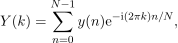
where ![k\in[0,N-1]](https://ima.org.uk/wp/wp-content/ql-cache/quicklatex.com-ad264a20b5c5459fa19021c4297e27fd_l3.svg "Rendered by QuickLaTeX.com") is the discrete frequency,
is the discrete frequency,  is the number of samples and
  is the signal value for sample
  . The output is then a discrete array of complex values across the frequency domain, which practically approximates the Fourier transform for a finite time series signal.
If we wish to understand how the spectral (frequency) content of a signal changes across the duration of the signal, we compute multiple DFTs. This approach is known as a short-time Fourier transform (STFT):
(3) 
where  represents the time step index of the STFT,
  is the hop size and
  is a window function of length . The output is now a discrete array of complex values across the time and frequency domains.
The window function can take several forms and is applied to the signal to avoid spectral leakage from discontinuities in the segmented time series data. The hop size is the number of samples the window shifts over for each frame of the STFT; this is usually set such that the frames overlap, which ensures that no time-domain information is lost. This procedure is illustrated in Figure 1.
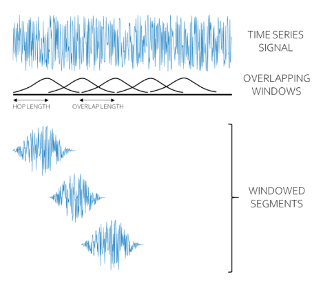
A typical choice for windowing parameters in audio signal processing is 75% overlap and, as adopted in this analysis, a periodic (sinusoidal) Hann window of length 128 samples.
To visualise the STFT of a time signal, we plot the magnitude  against both time and frequency. These plots are referred to as spectrograms, and they show how the amplitude (colour intensity) of the output changes with both time (x-axis) and frequency (y-axis).
European goldfinch example
The European goldfinch (Figure 2) is a beautiful bird, visually identified by its striking yellow wing patch, black tail and cherry red face. You might see them acrobatically foraging seeding plants, skillfully putting their pointed bills to good use. We will use a goldfinch song recording¹ as an example. This goldfinch song contains many trills, fast clicks and sweeping sounds, making it perfect for this visualisation exercise.

We adopt the STFT method to analyse an 11-second audio recording while varying the processing parameters to assess their impact on the method. The frequency resolution  of the STFT is related to the choice of DFT length
  and the sample frequency resolution
  according to
(4) 
With a sample frequency of 44 100 Hz (a typical audio sample frequency for smartphones), equation (4) then gives the following STFT resolutions for the spectrograms shown in Figure 3, which compares four combinations of DFT length and window length  :
:
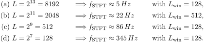
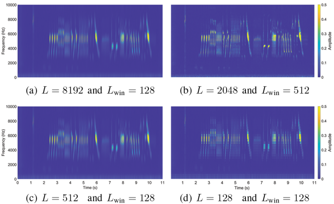
Increasing the DFT length improves the frequency resolution of the STFT output, leading to greater fidelity in the (frequency) y-axis. Compare, for example, spectrograms (a) and (d). However, increasing the DFT length also necessitates greater processing capability (to perform the analysis in a fixed time).
Therefore, if we wish to apply a real-time classification algorithm, we need to balance the fidelity of the output against the processing power and analysis time requirements. There are, however, many techniques to improve the performance of classification algorithms that are not memory intensive.
First, we will explore adjusting the STFT window length. For a fixed window overlap, increasing the STFT window length reduces the number of time steps in the STFT, which reduces the fidelity of the (time) x-axis. This also reduces the processing time, so that we can tune the DFT length and STFT window length together to balance the processing capability with both the frequency and time resolution.
For example, the frequency resolution of spectrogram (b) is a factor of 4 better than that for spectrogram (c), but (b) was produced using an extended window length. This sacrifices some time resolution but maintains the same processing time without losing the main temporal characteristics of the signal.
When classifying birds from recorded audio, it is typical to tune the parameters such that the time resolution is less than or equal to the minimum syllable length of an individual chirp (about 50 milliseconds). In our example, spectrogram (b) achieves a time resolution of 3 milliseconds, while (c) has a time resolution of <1 millisecond. This suggests that the settings used for (b) would be more than sufficient to balance the temporal and spectral characteristics of interest.
Continuous wavelet transforms
To overcome the challenges of balancing the time and frequency resolution, we can consider alternative transforms. The continuous wavelet transform is one such alternative for a simultaneous time and frequency analysis.
As detailed in [1], the continuous wavelet transform (CWT) of a time series signal  is defined as
(5) 
where  is the wavelet,
  represents the complex conjugate, is time and
  is a scale parameter (analogous to frequency). Each wavelet transform is defined for multiple scales . Equation (5) shifts each scaled wavelet along the time series, resulting in coefficients for each wavelet scale at every time sample from the original signal (analogous to the sinusoidal decomposition in the Fourier transform). This avoids the time sampling challenges faced by STFT processing.
A wavelet function  must have zero mean, finite energy and satisfy the admissibility condition:
(6) 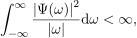
where  is the Fourier transform of and
  is the angular frequency. Wavelets that vanish for negative frequencies (i.e.,
  for
for  ) are analytic. For such transforms, (5) defines the analytic wavelet transform, which can be represented in the frequency domain as
(7) 
where  is the Fourier transform of the signal .
Wavelets are commonly defined as parameterised families. In this example, we will consider the Morse wavelet, defined in the frequency domain by
(8) 
where is the Heaviside function and  is a normalising constant. The time–bandwidth product
  and symmetry
  parameterise the shape of the wavelet.
By its very definition,  has a peak angular frequency. We can determine this by finding
  such that
(9) 
The natural logarithm of is more readily differentiated. For  :
:
(10) 
(11) 
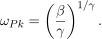
This gives  , so the peak angular frequency is
(12) 
By way of example, setting  and
and  gives a peak angular frequency
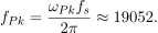
  , or equivalently for our audio signal,
(13) 
When undertaking a CWT analysis, the frequency domain is subdivided exponentially, each frequency being determined by the scale . This is parameterised by the number of voices per octave; the number of filters for each doubling of frequency. The scale spacing is, therefore, defined by
(14) 
where  is the scale index,
  is the number of voices per octave and
  is the base scale. Choosing
  , the scale spacing is
  . This represents a high value for
  and gives a fine frequency-domain spacing.
An example Morse wavelet  is shown in Figure 4. This shows the real and imaginary parts, with the magnitude of the wavelet in the time domain for scale
  (the total number of scales in this analysis is 770).
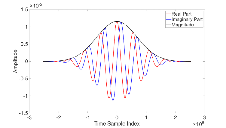
 700 with 48 voices per octave.
The exponential spacing of the frequency domain gives rise to fine resolution at low frequencies and coarse resolution at high frequencies. This, together with the finer resolution temporal output, makes the CWT well suited to fast transient sounds (3.5–4.0 seconds in the goldfinch recording) and ‘sweeps’, where a continuous sound varies in frequency over time (6.0 and 10.0 seconds in the goldfinch song recording).
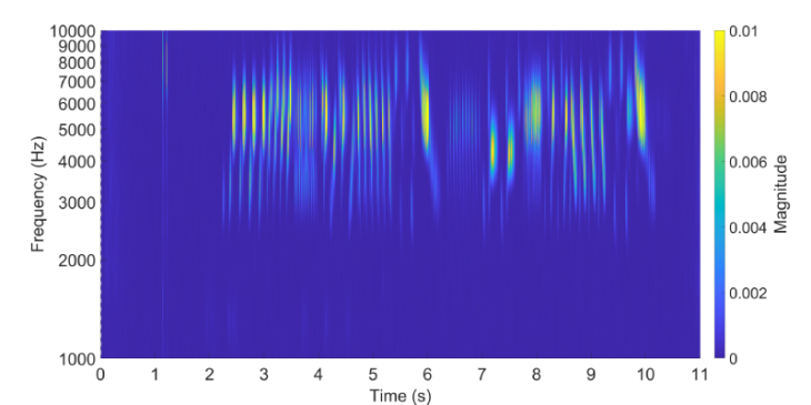
We can visualise the output of the CWT via a scalogram. This is like the spectrogram we encountered earlier, but it has a logarithmic y-axis to account for the non-uniform frequency scaling. Comparing Figure 5 with spectrogram (a), greater detail is revealed for fast transients and sweeps than realised with the STFT. The colour intensity scales of the spectrogram and scalogram have been set to ensure saturation at the higher amplitudes, which improves visualisation of the signals.
Conclusion
We have explored the mathematical foundations of two distinct signal processing methods, both of which enable visualisation of recorded audio signals. Taking this further, one could explore the benefits of each method for bird classification from recorded audio.
Convolutional neural networks are commonly used to identify patterns in two-dimensional visualisations, such as spectrograms and scalograms. The CWT has been shown to be more robust than the STFT when used as input to some classification tasks, for example, recognising faults in machinery from non-stationary acoustic signals [2].
Application of the CWT typically necessitates increased computational time (or additional processing capability) relative to the STFT. It is important to consider the processing time requirements; for example, an STFT-based method may be more appropriate for a remotely deployed near-real-time classification algorithm, whereas a CWT-based approach may yield more reliable results if an a posteriori analysis is acceptable.
Nathan Turner CMath FIMA
QinetiQ
Notes
- European goldfinch audio used with permission from Gregory Budney and the Macaulay Library.
References
- Lilly, J.M. and Olhede, S.C. (2010) On the analytic wavelet transform, IEEE Trans. Inf. Theory, vol. 56, no. 8, pp. 4135–4156.
- Phan, D.T. (2025) Comparison of short-time Fourier transform and wavelet transform as input data to convolutional neural networks for acoustical machinery fault recognition, Master’s thesis, Berliner Hochschule für Technik.
Reproduced from Mathematics Today, June 2026
Download the article, Birds on Holiday (pdf)