Since the 1890s, storytelling through moving images has gripped audiences across the globe. In post-war Britain, desperate to feel the magic of the big screen once again, people flocked to the cinema in record-breaking numbers. In 1946, 1.64 billion admissions were recorded in the UK [1]. [latexpage]
In a similar way, after nearly two years of disruption, cinemas expect to see admissions bounce back post-pandemic from their lowest numbers in at least eight decades. This is not surprising. Ultimately, whether it be by bracing for a jump scare, laugh-crying into our popcorn or swooning for actors that somehow meet impossible Hollywood beauty standards, a visit to the pictures is a way for us to enjoy ourselves and let loose. The stories that we are captivated by provide an entertaining distraction and a powerful form of escapism. As a species, we are enthralled by high-stakes adventures and dramatic portrayals.
Cinema is, of course, also a universal communicative tool. As well as livening up a Friday night, the stories told on the big screen can promote cultural understanding and comment on and challenge societal issues. Big screen storytelling has the power to inspire real change within our communities. After all, cinematic experiences are at the heart of the communal events we, maybe, took for granted before the pandemic. We share feelings, like the suspicion of Norman Bates when he talks about his mother, the frustration at how the door is definitely large enough to float Jack as well as Rose and the bittersweetness of an adorable alien finally ‘phoning home’. Now in the wake of the pandemic, getting the best movies back into our cinemas, so we can once again share in the moments of wonder, shock and awe, feels more important than ever.
Although we know mathematics has successfully elucidated many phenomena, art and mathematics can still seem unlikely partners. Among the things for which we do not yet have an exact formula is what makes a flick successful and beloved. What will satisfy audiences and then, of course, what will make money are the most pressing questions for a mathematician interested in turning their hand to the art of the big screen. When trying to understand the complex relationship between audiences and what they love, forecasting is a technique a mathematician has up their sleeve. In the following, we will be taking a quick tour through the forecasting models that can be applied to box office revenue prediction. We will be looking at the mathematical techniques that could help satisfy a deprived post-pandemic audience. In doing so, these methods aim to answer these crucial questions:
Do we have the next blockbuster?
Or just another box office flop?
First to premiere is multi-linear regression, which is a fundamental forecasting algorithm, falling into what are known as statistical learning methods. It works by fitting an equation between a dependent target variable and independent input variables that describe characteristics. In this context, the target variable $y$ is the box office earnings of a new motion picture. Input variables describe information about the new movie, such as the number of positive reviews, the value of the budget, box office revenue from the opening weekend and the number of mentions on Twitter. For $n$ input variables, the equation for the $i$th motion picture is given as follows:
\begin{equation*}
y_i = \beta_0 + \beta_1 x_{i1} + \beta_2 x_{i2} + \dots + \beta_n x_{in}
\end{equation*}
for $i = 1,2,\ldots,d$, where the $\beta$ values are regression coefficients. To obtain the regression coefficients, we can minimise the squared error between actual and predicted box office revenues [2]. Multi-linear regression can only capture linearity in the relationship between the independent features and the dependent target value but it can consider a wide range of influences on box office takings. In Figure 1, motion picture budget and online popularity are used to predict takings. The online popularity score is based on user interaction on The Movie Database website [3].
Figure 1: Multi-linear regression example using budget and online popularity obtained using data from The Movie Database [3].[/caption]
An alternative to multi-linear regression is to look at new product diffusion models, which are a type of time series forecasting model. The bass diffusion model [4] is especially popular and is not restricted by linearity. It considers two factors, innovation and imitation. The innovation parameter represents all mass media communication of the film. The imitation parameter explains responses of audiences that have already seen the movie and portrays the effect of word of mouth [5]. The model gives a hazard rate, which is the probability that a potential audience member who has not yet seen the film will watch it at time $t$. The hazard rate is given as:
\begin{equation*}
h(t) = \frac{N'(t)}{1-N(t)} = p + qN(t),
\end{equation*}
where $p$ is our innovation coefficient and $q$ is the imitation coefficient. $N(t)$ is the cumulative portion of potential moviegoers who have seen the film at time $t$, that is, the number of people who have seen the film by time $t$ out of all possible cinemagoers, $M$. $N'(t)$ is its derivative with respect to time. What the hazard rate tells us is that the portion of the potential moviegoers who go to see the film for the first time at time $t$ can be written as a linear function of the people who have already seen it.
The bass diffusion model differential equation is
\begin{equation*}
N'(t) = p + (q-p)N(t)-q[N(t)]^2.
\end{equation*}
At time $t = 0$, the cumulative proportion of the potential audience who have seen the film is zero. We can solve the differential equation and write $N(t)$ as
\begin{equation*}
N(t) = \frac{1-\operatorname{e}^{-(p + q)t}}{1 + (q/p )\operatorname{e}^{-(p + q)t}}.
\end{equation*}
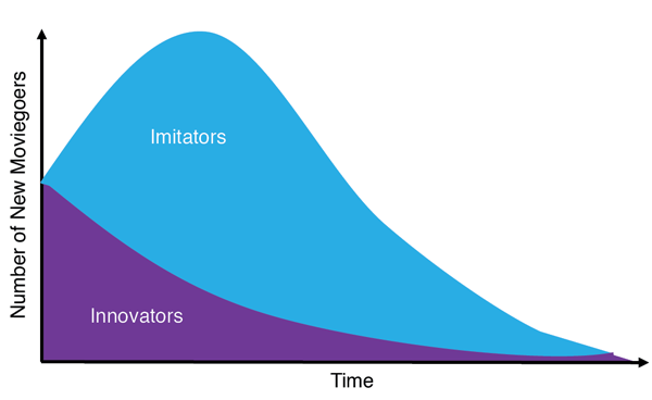
The model has three unknown parameters, which need to be estimated: the innovation parameter, the imitation parameter and the number of potential cinemagoers, $M$. The latter, $M$, can be estimated in a number of ways using historical data, such as total cinema admissions. As shown by Figure 2, when we look at the number of new moviegoers, we are effectively splitting the audience of a film into two categories: innovators and imitators. Innovation is what gives a movie its momentum from the get-go. These are the factors that entice audience members in from early on, whether that be studio reputation, advertising and promotions or just the presence of Tom Cruise. In practice, the box office takings from the opening weekend can usually be used to gain a reasonable estimate of $p$. Conversely, the imitation parameter needs to capture all the internal factors likely to get you off your couch and into the cinema, chomping on popcorn. This includes word of mouth as well as social media buzz. In reality, one possible way we could approximate this is by measuring the positivity of user reviews online.
Once we have $N(t)$ we can multiply by $M$ to get the cumulative number of people who will watch the film by time $t$. Using information about ticket revenue, we can calculate the predicted total box office figure. In Figure 3, a bass model offers to dispel the mystery around revenue for the whodunnit Knives Out [6]. Admissions for the blockbuster were halted on its 106th day, at the beginning of the pandemic.
Figure 3: Bass model fitted to box office revenue data for Knives Out [6]. Predictions given by the green line.[/caption]
Another option to model the expected revenue for a new motion picture is to venture into machine learning based regression algorithms such as the $k$-NN algorithm. It is favourable within its realm for its simplicity and the fact that it does not require a training procedure to be implemented. The $k$-NN process uses information about previous motion pictures and their corresponding box office takings. By looking at previous movies with similar features, $k$-NN utilises known box office earnings to forecast the success of a new release.
The first step is to calculate how similar the new release is to previous films. For instance, we could measure similarity based on characteristics such as budget and rating. One way to measure the distance between a film and a new release is to compute the Euclidean distance, the square roots of the sum of the squared difference between the new point and the existing points (after suitable normalisation). The set of the $k$ most similar films are selected and dubbed the ‘nearest neighbours’. For each of the nearest neighbours, the box office takings, $y_j$, are observed and weights, $w_j$, are assigned.
Figure 4: Example of k-NN performed using data from The Movie Database [3]. Predictions given by the green line.[/caption]
The predicted box office earnings for a new release $i$ are given as the following [2]:
\begin{equation*}
\widehat{y}_i = \sum_{j\in k-NN(x_i)}w_j y_j.
\end{equation*}
Figure 4 shows $k$-NN predictions using online popularity [3].
To execute $k$-NN, the number of neighbours and the weights assigned to those neighbours need to be chosen. The number of neighbours, $k$, is often chosen by cross-validating empirical evidence. When it comes to the weights, it feels logical to assign a neighbour that is further away a smaller weight than a neighbour that is closer. This commonly leads to the adoption of some kind of kernel function, which monotonically decreases as distance increases [7].
Support vector regression [8] is also an algorithm to be considered. It is a nonlinear regression algorithm that works by fitting the equation $\widehat{y} = \boldsymbol{w}^{\boldsymbol{T}} \boldsymbol{x} + b$ using a training sample comprising motion picture features and known box office takings. In Figure 5, motion picture budget is used.
Figure 5: Example of support vector regression performed using data from The Movie Database [3]. Predictions given in green.[/caption]
The aim is to consider points within a boundary. We want the hyperplane that includes the maximum number of points whilst also looking to minimise error, $\epsilon$. To get a flat function, we want a small $\boldsymbol{w}$ so we minimise the norm, $\frac{1}{2}\|\boldsymbol{w}\|^2$. The fitting of the regression equation can be modelled as the convex optimisation problem:
\begin{align*}
\min \frac{1}{2}\big|\big|\boldsymbol{w}\big|\big|^2 &+ C\sum_{i = 1}^n(\xi_i + \xi_i^*)\
\text{s.t.} \quad y_i = \boldsymbol{w}^T\boldsymbol{x} + b &\le \epsilon + \xi_i\
\boldsymbol{w}^T\boldsymbol{x} + b - y_i &\le \epsilon + \xi_i^*\
\xi_i,\xi_i^* &\ge 0.
\end{align*}
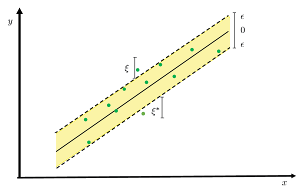
In this formulation, there are added slack variables, $\xi_i$ and $\xi_i^*$. These are helpful because a function that approximates all pairs within $\epsilon$ might not exist. As illustrated by Figure 6, it may be useful to allow for some error.
We then have a trade-off between flatness and the errors that we want to allow. We could opt for a function as flat as possible, setting $C$ to a very small value, but then our observations will have greater errors. If, instead, we want to focus on having very small errors, we can set $C$ to a large value but then flatness will take a back seat, as the shape of the regression function will need to capture a large number of the observations. In support vector regression, it is important to balance getting accurate box office forecasts and having a function that is not so complicated that it loses generality.
And that is a wrap! Although predicting the success of art, and how to satisfy worldwide audiences, is an inherently complicated task, mathematicians are not completely helpless. Using forecasting algorithms, mathematics and storytelling can come together with the aim of maximising audience gratification. As cinemas get back on their feet and it feels safe once again to journey into alternative universes and join breathtaking adventures, we can only hope that box office hits are all that lie in store for the patient audiences who have longed for their return to the big screen.
UK Cinema Association (2021) UK Cinema Admissions and Box Office, Annual Admissions.
Kim, T., Hong, J. and Kang, P. (2015) Box office forecasting using machine learning algorithms based on SNS data, Int. J. Forecasting, vol. 31, no. 2, pp. 364–390.
Bass, F. (1969) A new product growth for model consumer durables, Manage. Sci., vol. 15, no. 5, pp. 215–227.
Dellarocas, C., Zhang, X. and Awad, N. (2007) Exploring the value of online product reviews in forecasting sales: The case of motion pictures, J. Interact. Mark., vol. 21, no. 4, pp. 23–45.
Box Office Mojo (2021) Knives Out.
Kang, P. and Cho, S. (2008) Locally linear reconstruction for instance-based learning, Pattern Recognit., vol. 41, no. 11, pp. 3507–3518.
Smola, A. and Schölkopf, B. (2004) A tutorial on support vector regression, Stat. Comput., vol. 14, no. 3, pp. 199–222.

![Figure 1: Multi-linear regression example using budget and online popularity obtained using data from The Movie Database [3].](https://ima.org.uk/static/3359fb7df217a5c232e0b32cc0e69711/482x412_highestquality__4a7c7e45a350/Figure-1-Multi-linear-regression-example-using-budget-and-online-popularity-obtained-using-data-from-The-Movi.png) Figure 1: Multi-linear regression example using budget and online popularity obtained using data from The Movie Database [3].[/caption]
An alternative to multi-linear regression is to look at new product diffusion models, which are a type of time series forecasting model. The bass diffusion model [4] is especially popular and is not restricted by linearity. It considers two factors, innovation and imitation. The innovation parameter represents all mass media communication of the film. The imitation parameter explains responses of audiences that have already seen the movie and portrays the effect of word of mouth [5]. The model gives a hazard rate, which is the probability that a potential audience member who has not yet seen the film will watch it at time $t$. The hazard rate is given as:
\begin{equation*}
h(t) = \frac{N'(t)}{1-N(t)} = p + qN(t),
\end{equation*}
where $p$ is our innovation coefficient and $q$ is the imitation coefficient. $N(t)$ is the cumulative portion of potential moviegoers who have seen the film at time $t$, that is, the number of people who have seen the film by time $t$ out of all possible cinemagoers, $M$. $N'(t)$ is its derivative with respect to time. What the hazard rate tells us is that the portion of the potential moviegoers who go to see the film for the first time at time $t$ can be written as a linear function of the people who have already seen it.
The bass diffusion model differential equation is
\begin{equation*}
N'(t) = p + (q-p)N(t)-q[N(t)]^2.
\end{equation*}
At time $t = 0$, the cumulative proportion of the potential audience who have seen the film is zero. We can solve the differential equation and write $N(t)$ as
\begin{equation*}
N(t) = \frac{1-\operatorname{e}^{-(p + q)t}}{1 + (q/p )\operatorname{e}^{-(p + q)t}}.
\end{equation*}
Figure 1: Multi-linear regression example using budget and online popularity obtained using data from The Movie Database [3].[/caption]
An alternative to multi-linear regression is to look at new product diffusion models, which are a type of time series forecasting model. The bass diffusion model [4] is especially popular and is not restricted by linearity. It considers two factors, innovation and imitation. The innovation parameter represents all mass media communication of the film. The imitation parameter explains responses of audiences that have already seen the movie and portrays the effect of word of mouth [5]. The model gives a hazard rate, which is the probability that a potential audience member who has not yet seen the film will watch it at time $t$. The hazard rate is given as:
\begin{equation*}
h(t) = \frac{N'(t)}{1-N(t)} = p + qN(t),
\end{equation*}
where $p$ is our innovation coefficient and $q$ is the imitation coefficient. $N(t)$ is the cumulative portion of potential moviegoers who have seen the film at time $t$, that is, the number of people who have seen the film by time $t$ out of all possible cinemagoers, $M$. $N'(t)$ is its derivative with respect to time. What the hazard rate tells us is that the portion of the potential moviegoers who go to see the film for the first time at time $t$ can be written as a linear function of the people who have already seen it.
The bass diffusion model differential equation is
\begin{equation*}
N'(t) = p + (q-p)N(t)-q[N(t)]^2.
\end{equation*}
At time $t = 0$, the cumulative proportion of the potential audience who have seen the film is zero. We can solve the differential equation and write $N(t)$ as
\begin{equation*}
N(t) = \frac{1-\operatorname{e}^{-(p + q)t}}{1 + (q/p )\operatorname{e}^{-(p + q)t}}.
\end{equation*}
 The model has three unknown parameters, which need to be estimated: the innovation parameter, the imitation parameter and the number of potential cinemagoers, $M$. The latter, $M$, can be estimated in a number of ways using historical data, such as total cinema admissions. As shown by Figure 2, when we look at the number of new moviegoers, we are effectively splitting the audience of a film into two categories: innovators and imitators. Innovation is what gives a movie its momentum from the get-go. These are the factors that entice audience members in from early on, whether that be studio reputation, advertising and promotions or just the presence of Tom Cruise. In practice, the box office takings from the opening weekend can usually be used to gain a reasonable estimate of $p$. Conversely, the imitation parameter needs to capture all the internal factors likely to get you off your couch and into the cinema, chomping on popcorn. This includes word of mouth as well as social media buzz. In reality, one possible way we could approximate this is by measuring the positivity of user reviews online.
Once we have $N(t)$ we can multiply by $M$ to get the cumulative number of people who will watch the film by time $t$. Using information about ticket revenue, we can calculate the predicted total box office figure. In Figure 3, a bass model offers to dispel the mystery around revenue for the whodunnit Knives Out [6]. Admissions for the blockbuster were halted on its 106th day, at the beginning of the pandemic.
The model has three unknown parameters, which need to be estimated: the innovation parameter, the imitation parameter and the number of potential cinemagoers, $M$. The latter, $M$, can be estimated in a number of ways using historical data, such as total cinema admissions. As shown by Figure 2, when we look at the number of new moviegoers, we are effectively splitting the audience of a film into two categories: innovators and imitators. Innovation is what gives a movie its momentum from the get-go. These are the factors that entice audience members in from early on, whether that be studio reputation, advertising and promotions or just the presence of Tom Cruise. In practice, the box office takings from the opening weekend can usually be used to gain a reasonable estimate of $p$. Conversely, the imitation parameter needs to capture all the internal factors likely to get you off your couch and into the cinema, chomping on popcorn. This includes word of mouth as well as social media buzz. In reality, one possible way we could approximate this is by measuring the positivity of user reviews online.
Once we have $N(t)$ we can multiply by $M$ to get the cumulative number of people who will watch the film by time $t$. Using information about ticket revenue, we can calculate the predicted total box office figure. In Figure 3, a bass model offers to dispel the mystery around revenue for the whodunnit Knives Out [6]. Admissions for the blockbuster were halted on its 106th day, at the beginning of the pandemic.
![Figure 3: Bass model fitted to box office revenue data for Knives Out [6]. Predictions given by the green line.](https://ima.org.uk/static/290f0f100fc2c249ac0b6971a4c0d4dd/600x262_highestquality__4a7c7e45a350/Figure-3-Bass-model-fitted-to-box-office-revenue-data-for-Knives-Out-6-Predictions-given-by-the-green-line.png) Figure 3: Bass model fitted to box office revenue data for Knives Out [6]. Predictions given by the green line.[/caption]
Another option to model the expected revenue for a new motion picture is to venture into machine learning based regression algorithms such as the $k$-NN algorithm. It is favourable within its realm for its simplicity and the fact that it does not require a training procedure to be implemented. The $k$-NN process uses information about previous motion pictures and their corresponding box office takings. By looking at previous movies with similar features, $k$-NN utilises known box office earnings to forecast the success of a new release.
The first step is to calculate how similar the new release is to previous films. For instance, we could measure similarity based on characteristics such as budget and rating. One way to measure the distance between a film and a new release is to compute the Euclidean distance, the square roots of the sum of the squared difference between the new point and the existing points (after suitable normalisation). The set of the $k$ most similar films are selected and dubbed the ‘nearest neighbours’. For each of the nearest neighbours, the box office takings, $y_j$, are observed and weights, $w_j$, are assigned.
Figure 3: Bass model fitted to box office revenue data for Knives Out [6]. Predictions given by the green line.[/caption]
Another option to model the expected revenue for a new motion picture is to venture into machine learning based regression algorithms such as the $k$-NN algorithm. It is favourable within its realm for its simplicity and the fact that it does not require a training procedure to be implemented. The $k$-NN process uses information about previous motion pictures and their corresponding box office takings. By looking at previous movies with similar features, $k$-NN utilises known box office earnings to forecast the success of a new release.
The first step is to calculate how similar the new release is to previous films. For instance, we could measure similarity based on characteristics such as budget and rating. One way to measure the distance between a film and a new release is to compute the Euclidean distance, the square roots of the sum of the squared difference between the new point and the existing points (after suitable normalisation). The set of the $k$ most similar films are selected and dubbed the ‘nearest neighbours’. For each of the nearest neighbours, the box office takings, $y_j$, are observed and weights, $w_j$, are assigned.
![Figure 4: Example of k-NN performed using data from The Movie Database [3]. Predictions given by the green line.](https://ima.org.uk/static/a408bf6e098dcaf595a3b787b37bfd2b/600x261_highestquality__4a7c7e45a350/Figure-4-Example-of-k-NN-performed-using-data-from-The-Movie-Database-3-Predictions-given-by-the-green-lin.png) Figure 4: Example of k-NN performed using data from The Movie Database [3]. Predictions given by the green line.[/caption]
The predicted box office earnings for a new release $i$ are given as the following [2]:
\begin{equation*}
\widehat{y}_i = \sum_{j\in k-NN(x_i)}w_j y_j.
\end{equation*}
Figure 4 shows $k$-NN predictions using online popularity [3].
To execute $k$-NN, the number of neighbours and the weights assigned to those neighbours need to be chosen. The number of neighbours, $k$, is often chosen by cross-validating empirical evidence. When it comes to the weights, it feels logical to assign a neighbour that is further away a smaller weight than a neighbour that is closer. This commonly leads to the adoption of some kind of kernel function, which monotonically decreases as distance increases [7].
Support vector regression [8] is also an algorithm to be considered. It is a nonlinear regression algorithm that works by fitting the equation $\widehat{y} = \boldsymbol{w}^{\boldsymbol{T}} \boldsymbol{x} + b$ using a training sample comprising motion picture features and known box office takings. In Figure 5, motion picture budget is used.
Figure 4: Example of k-NN performed using data from The Movie Database [3]. Predictions given by the green line.[/caption]
The predicted box office earnings for a new release $i$ are given as the following [2]:
\begin{equation*}
\widehat{y}_i = \sum_{j\in k-NN(x_i)}w_j y_j.
\end{equation*}
Figure 4 shows $k$-NN predictions using online popularity [3].
To execute $k$-NN, the number of neighbours and the weights assigned to those neighbours need to be chosen. The number of neighbours, $k$, is often chosen by cross-validating empirical evidence. When it comes to the weights, it feels logical to assign a neighbour that is further away a smaller weight than a neighbour that is closer. This commonly leads to the adoption of some kind of kernel function, which monotonically decreases as distance increases [7].
Support vector regression [8] is also an algorithm to be considered. It is a nonlinear regression algorithm that works by fitting the equation $\widehat{y} = \boldsymbol{w}^{\boldsymbol{T}} \boldsymbol{x} + b$ using a training sample comprising motion picture features and known box office takings. In Figure 5, motion picture budget is used.
![Figure 5: Example of support vector regression performed using data from The Movie Database [3]. Predictions given in green.](https://ima.org.uk/static/554d51bace50407ccf52f68dda9782d3/600x258_highestquality__4a7c7e45a350/Figure-5-Example-of-support-vector-regression-performed-using-data-from-The-Movie-Database-3-Predictions-g.png) Figure 5: Example of support vector regression performed using data from The Movie Database [3]. Predictions given in green.[/caption]
The aim is to consider points within a boundary. We want the hyperplane that includes the maximum number of points whilst also looking to minimise error, $\epsilon$. To get a flat function, we want a small $\boldsymbol{w}$ so we minimise the norm, $\frac{1}{2}\|\boldsymbol{w}\|^2$. The fitting of the regression equation can be modelled as the convex optimisation problem:
\begin{align*}
\min \frac{1}{2}\big|\big|\boldsymbol{w}\big|\big|^2 &+ C\sum_{i = 1}^n(\xi_i + \xi_i^*)\
\text{s.t.} \quad y_i = \boldsymbol{w}^T\boldsymbol{x} + b &\le \epsilon + \xi_i\
\boldsymbol{w}^T\boldsymbol{x} + b - y_i &\le \epsilon + \xi_i^*\
\xi_i,\xi_i^* &\ge 0.
\end{align*}
In this formulation, there are added slack variables, $\xi_i$ and $\xi_i^*$. These are helpful because a function that approximates all pairs within $\epsilon$ might not exist. As illustrated by Figure 6, it may be useful to allow for some error.
Figure 5: Example of support vector regression performed using data from The Movie Database [3]. Predictions given in green.[/caption]
The aim is to consider points within a boundary. We want the hyperplane that includes the maximum number of points whilst also looking to minimise error, $\epsilon$. To get a flat function, we want a small $\boldsymbol{w}$ so we minimise the norm, $\frac{1}{2}\|\boldsymbol{w}\|^2$. The fitting of the regression equation can be modelled as the convex optimisation problem:
\begin{align*}
\min \frac{1}{2}\big|\big|\boldsymbol{w}\big|\big|^2 &+ C\sum_{i = 1}^n(\xi_i + \xi_i^*)\
\text{s.t.} \quad y_i = \boldsymbol{w}^T\boldsymbol{x} + b &\le \epsilon + \xi_i\
\boldsymbol{w}^T\boldsymbol{x} + b - y_i &\le \epsilon + \xi_i^*\
\xi_i,\xi_i^* &\ge 0.
\end{align*}
In this formulation, there are added slack variables, $\xi_i$ and $\xi_i^*$. These are helpful because a function that approximates all pairs within $\epsilon$ might not exist. As illustrated by Figure 6, it may be useful to allow for some error.
 We then have a trade-off between flatness and the errors that we want to allow. We could opt for a function as flat as possible, setting $C$ to a very small value, but then our observations will have greater errors. If, instead, we want to focus on having very small errors, we can set $C$ to a large value but then flatness will take a back seat, as the shape of the regression function will need to capture a large number of the observations. In support vector regression, it is important to balance getting accurate box office forecasts and having a function that is not so complicated that it loses generality.
And that is a wrap! Although predicting the success of art, and how to satisfy worldwide audiences, is an inherently complicated task, mathematicians are not completely helpless. Using forecasting algorithms, mathematics and storytelling can come together with the aim of maximising audience gratification. As cinemas get back on their feet and it feels safe once again to journey into alternative universes and join breathtaking adventures, we can only hope that box office hits are all that lie in store for the patient audiences who have longed for their return to the big screen.
We then have a trade-off between flatness and the errors that we want to allow. We could opt for a function as flat as possible, setting $C$ to a very small value, but then our observations will have greater errors. If, instead, we want to focus on having very small errors, we can set $C$ to a large value but then flatness will take a back seat, as the shape of the regression function will need to capture a large number of the observations. In support vector regression, it is important to balance getting accurate box office forecasts and having a function that is not so complicated that it loses generality.
And that is a wrap! Although predicting the success of art, and how to satisfy worldwide audiences, is an inherently complicated task, mathematicians are not completely helpless. Using forecasting algorithms, mathematics and storytelling can come together with the aim of maximising audience gratification. As cinemas get back on their feet and it feels safe once again to journey into alternative universes and join breathtaking adventures, we can only hope that box office hits are all that lie in store for the patient audiences who have longed for their return to the big screen.